Independence and dependence
What can be computed in parallel?
Suppose we have a sequential computation (a sequence of operations or instructions) that we need to execute:
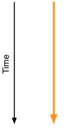
Could we perhaps split this sequential computation into multiple parts that we could then execute in parallel, to finish the computation faster?
Clearly we cannot do this for an arbitrary computation, since the next operation in a sequence of operations may depend on the outcome of the current operation, and hence the next operation cannot be started before the result of the current operation is available.
But what are the rules in this quest for parallelism?
What precisely can be computed in parallel?
A functional perspective
Let us adopt a simplified, functional perspective to program execution. In particular, let us view each “operation” as an application of a pure function to some values.
That is, an execution is a sequence of values, where the current value is obtained by applying a pure function to previous values in the sequence:
Here you may think of the pure functions as anything ranging between very simple functions (say, single processor instructions) to something complex but which can still be viewed as a pure function (say, a database query executed via multiple network services but whose result depends only on the parameters of the query).
Within this simplified perspective, let us now look at examples of sequential executions and think whether we can execute them in parallel.
Independence
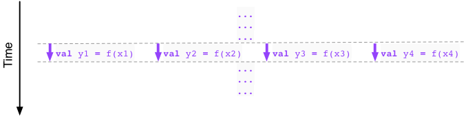
Here is our first example:
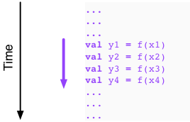
We observe that the four applications of the function f use values
x1, x2, x3, x4 that are already available to us,
courtesy of the execution thus far (indicated by “...”).
So there is nothing (that is, no dependence between the values)
that would prevent us from executing the function applications
in parallel, independently of each other:
In particular, we can in principle run this part of our program
four times as fast by scheduling the four independent applications
of f in parallel. In practice the speedup may be less substantial
(see warning box below).
Note
Observe that executions such as our example above are rather
typical in functional programming style. That is, we are in
effect mapping the function f over independent values
(x1, x2, x3, x4) to
yield a new sequence of values (y1, y2, y3, y4).
This type of parallelism is frequently called applying a
single instruction (that is, “f”)
to multiple (independent) data items, or SIMD parallelism.
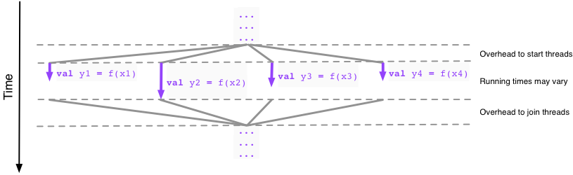
Warning
While SIMD parallelism at low level (in particular, when implemented
in hardware) can and often does yield speedup over sequential execution
that is proportional to the number of independent data items, at higher
level the speedup is often less substantial. This is because there
is typically some overhead to start and stop parallel execution
(e.g. start and join threads), and our function f may have complex
internal structure that causes the running times to vary between different
data items:
A further caveat to speedup obtained by SIMD parallelism is the availability of data in the memory hierarchy. For example, low bandwidth to main memory may eliminate SIMD parallel speedup in memory-intensive applications.
Dependence
Let us now look at a second example. Here we go:
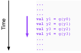
Now it looks like we are in trouble. Indeed, to compute y2
we must have available y1, to compute y3 we must have
available y2, and to compute y4 we must have available y3.
It appears that there is nothing we can do here. That is,
we must first evaluate y1, then y2, then y3, and then y4,
with no possibility to execute any of the evaluations in parallel.
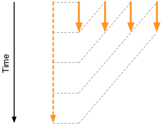
Such a situation is common in iterative computations where the
next value depends on the current value (and all previous values).
This happens, for example, when we are running a simulation
that proceeds in discrete time steps, such as our tick-by-tick
armlet simulation from Module I: The mystery of the computer.
Modelling dependence with directed acyclic graphs (DAGs)
Our two previous examples were two extremes. At one extreme, we have complete independence, with linear speedup by parallelization (subject to caveats in the warning box above). At the other extreme, we have complete dependence and no possibility to obtain speedup by parallelization (subject to caveats in the warning boxes further below).
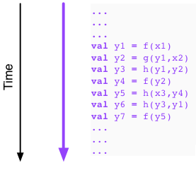
Let us next look at an example in between the two extreme cases:
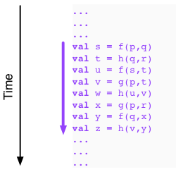
We can illustrate the dependencies between the functions by building a directed graph from the example above. Drawing a directed edge from values to functions dependent on them:
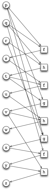
On the left, we have the values (indicated by circular nodes) in the computation; on the right, we have the functions (indicated by square nodes) that are applied to values (indicated by incoming edges) to yield a new value (indicated by outgoing edge).
Observe that we have intentionally drawn the directed graph in such a way that ordering of the nodes reflects the progress of time in the sequential computation. In particular, all edges are oriented (diagonally) from top to bottom, in the direction of time in the original figure. It follows that the directed graph has no cycles. Thus, we have in fact a directed acyclic graph (a DAG).
We also observe that the DAG above is in fact essentially a complete representation of the sequential computation in the example. Indeed, the only information that is missing from the DAG is the order in which the parameters are given to the functions (that is, which of the incoming values to a function is the first parameter, which the second, and so forth); if necessary we could indicate this by labelling the incoming edges to a function with ordinals, but we choose not to do this for simplicity.
This DAG representation is convenient because it captures the dependence between values. In particular, a value \(j\) depends on another value \(i\) if and only if there is a directed path from \(i\) to \(j\) in the DAG. It follows immediately that we can use the DAG to investigate whether we can carry out parts of (or all of) the computation represented by the DAG in parallel.
In practice we can carry out such an investigation by partitioning the nodes of the DAG into (topological) levels so that the nodes at level \(0\) are precisely the nodes with no incoming edges, and the nodes at level \(\ell=1,2,\ldots\) are precisely the nodes with at least one incoming edge from a node at level \(\ell-1\). (That is, the nodes at level \(\ell\) are precisely the nodes that have no incoming edges if we delete the nodes at levels \(0,1,\ldots,\ell-1\). That is, the level of a node is the number of edges in the longest directed path in the DAG that ends at the node.)
Here is the example DAG partitioned into levels:
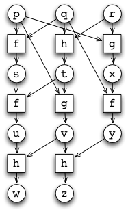
This partitioning immediately suggests that we can execute the example computation in parallel using multiple threads.
Remark. (*) An interested reader may want to take a look at topological sorting of DAGs.
Minimum makespan and scheduling
If we associate with each function node in the DAG the time it takes to compute the value of the function with the indicated parameter values, we observe that the longest directed path of nodes in the DAG (where the length is measured by the sum of the times associated with the function nodes in the path) is the minimum makespan of the computation.
That is, the minimum makespan is the minimum amount of time it takes to finish the computation if we have access to sufficient parallel computing resources to execute all relevant function evaluations in parallel. In fact, assuming furthermore that there is no time overhead to start and join threads, the minimum makespan is achieved simply by starting each function evaluation in its own thread as soon as its parameter values are available. In particular this can be done without knowing how long it takes to execute each function evaluation.
(This observation is in fact the design rationale for the Future abstraction that we will discuss in what follows.)
Warning
In practice there is of course a limit on the amount of parallel computing resources available, so scheduling each function evaluation in its own thread as soon as its parameter values are available may not be possible. Furthermore, in practice there is overhead in starting, joining, and synchronizing threads, so even if one could schedule everything in parallel, this may not be efficient because of the overhead involved.
Remark. (**) An interested reader may want to take a look at the critical path method and scheduling more generally, or, say, in the context of job shop scheduling.
Parallel speedup and Amdahl’s law
While in some cases it is possible to reduce the time it takes to complete a sequential computation by executing parts of the computation in parallel, a fact observed in practice is that our programs contain sequential parts that we do not know how to parallelize.
Such sequentialism in our programs limits the possible parallel speedup (the ratio of the computation time without taking advantage of parallelism to the computation time when taking advantage of parallelism) obtainable by deploying additional parallel processors to execute our program. In more precise terms, if we can take advantage of parallelism only in a \(P\)-portion of our program, \(0\leq P<1\), then the parallel speedup is bounded from above by \(1/(1-P)\) no matter how many parallel processors we have available and even if there is no overhead.
This practical limit to parallel speedup is known as Amdahl’s argument or Amdahl’s law (follow the link for a justification of the \(1/(1-P)\) upper bound).
What can be computed in parallel, revisited
We have now obtained some insight into what can be computed more efficiently if we have access to parallel resources by resorting to a simplified, functional model of sequential computation. We should, however, recognize that this model is rather pedestrian.
Indeed, the limits of our model are revealed already when we look at the task of computing a sum of multiple integer values, say, suppose we want to compute a sum
where \(p,q,r,s,t,u,v,w\) are integers.
If we now select an unfortunate sequential implementation for the sum, and view addition of two values \(a,b\) as a function \((a,b)\mapsto f(a,b)=a+b\), from the perspective of our model it quickly looks as if there is nothing we could do because of sequential dependence between the values \(y_1,y_2,\ldots,y_6,z\):
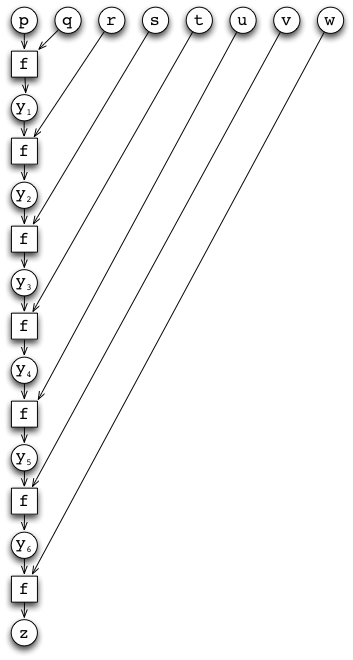
On the surface of it, it looks like we are in serious trouble indeed.
However, this dependence is in fact model-induced and not as bad as it looks because addition is associative. That is, we have
Because of associativity we could have just as well chosen our sequential computation to be:
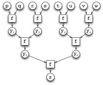
Suddenly it appears that there is no problem at all to obtain parallel speedup for sums.
Remark. Assuming we have \(n\) parallel processors and no overhead for parallelization, we can take the sum of \(n\) integers in time \(\mathcal{O}(\log n)\) by structuring the dependence DAG as a perfect binary tree. (Above we see the case \(n=8\).)
Warning
It is, in fact, in most cases not at all immediate how we should make use of parallel resources if we want to get something done so that we make optimal use of these resources. The example of addition and the apparent dependence indicated by our functional model should be viewed as a positive warning in this regard.
Note
Associativity is a useful property shared by many mathematical operators, such as integer addition, product, maximum, and minimum. In fact, all expressions constructed using an associative operator (such as the sum above) can be computed efficiently in parallel by structuring the dependency DAG as a perfect binary tree.
Warning
Not all mathematical operators are associative. For example, integer subtraction and division are not associative.
In concrete programming terms, we will encounter the serendipity of associativity in the context of the Scala parallel collections framework, to be considered next. Indeed, now it is about time to proceed to the gains of all this reading effort.