Efficiency
CS-A1120 Programming 2
Lukas Ahrenberg
Department of Computer Science
Aalto University
After this round, you
- can provide examples of computational resources
- can measure program run-time in Scala
- know the mathematical definitions of \(\mathcal{O}\), \(\Omega\), and \(\Theta\)
- can define Big-O for program running times, and
- analyse a basic program in this respect
- have experience of indexing and searching
- can implement and use binary search
Efficiency ?
- Why does the efficiency of a program matter?
- How can it be defined?
- How can it be measured?
Discuss and let us know https://presemo.aalto.fi/prog2

Efficiency aim
We want the amount of resources necessary to complete a task to scale well when the input instance grows in size.
- In practice:
- The exam papers (for grading, scales with the number of students)
- An image (for processing, scales with resolution)
- A matrix (for calculations, scales with number of entries)
Computation requires resources
- Time
- Space
- Memory
- Storage
- Energy
- Bandwidth
- Processors
- …
Time
- In this course we will (mostly) focus on time efficiency
- Not only about waiting: each clock 'tick' of the CPU typically costs energy
- How can we reason about the time it takes to run a specific program?
- Measure it
- Analyse the code
- Analyse the algorithm
- How can we improve the run–time of some piece of code?
- Increase resources (more/faster hardware)
- Optimise the code
- Implement a better performing algorithm
Measuring the running time
Different ways of measuring the running time of a program:
- Wall clock time (= Elapsed time) : time measured by an "external clock" (Note that if there are other resource intensive programs running on the computer the measured program needs to wait.)
- CPU time: time spent by the CPU running the program, subdivided into
- User time: time that is spent on the program code
- System time: time that is spent on system calls made by the program (I/O, etc)
In the following we will focus on measuring CPU time.
Measuring CPU time in Scala
// Import from Java
import java.lang.management.{ManagementFactory,
  ThreadMXBean}
// Set-up
val bean: ThreadMXBean = ManagementFactory
  .getThreadMXBean()

// Get time, or 0 if functionality not supported
def getCpuTime: Long =
  if bean.isCurrentThreadCpuTimeSupported() then
    bean.getCurrentThreadCpuTime()
  else
    0L
def measureCpuTime[T](f: => T): (T, Double) =
  val start: Long = getCpuTime
  val r = f
  val end: Long = getCpuTime
  val t: Double = (end - start) / 1e9
  (r, t)
measureCpuTime:getCPUTime- Execute function (
fis call-by-name) getCPUTime- Calculate difference
- Measuring once, good enough if we think the operation will take more than about 0.1 s
- Some caveats on windows with small running times
- Using ThreadMXBean from for CPU Time:
- nanosecond precision but not accuracy
Measuring how long time it takes to add up \(n\) numbers
// Our summation of values from 1 to n
def f(m: Long): Long =
  var i = 1L
  var s = 0L
  while i <= m do
    s = s + i
    i = i + 1
  s
// Time for all n in this sequence
val ns = Seq(1000000000L, 2000000000L,
  3000000000L, 4000000000L)
// Perform measurement for each n in ns
val fData = ns.map(n => measureCpuTime( f(n) ) )
After running the above measurement in a Scala REPL on a laptop we have the following values in fData (word-wrapped for readability):
scala> fData
val res: Seq[(Long, Double)] = List(
  (500000000500000000,0.23691685),
  (2000000001000000000,0.469175766),
  (4500000001500000000,0.787165003),
  (8000000002000000000,1.017464763))
These can be plotted to give us a hint of how running time depends on \(n\).
A more advanced example: Matrix operations
In our case \(n \times n\) square matrices, e.g. \[ A = \begin{pmatrix} a_{(0,0)} & a_{(0,1)} & \cdots & a_{(0,n-1)}\\ a_{(1,0)} & a_{(1,1)} & \cdots & a_{(1,n-1)}\\ \vdots & \vdots & \ddots & \vdots\\ a_{(n-1,0)} & a_{(n-1,1)} & \cdots & a_{(n-1,n-1)} \end{pmatrix} \]
Matrix sum and multiplication
\(C = A + B\)
Per element:
\(c_{(i,j)} = a_{(i,j)} + b_{(i,j)}\)
For example:
\(C = A B\)
Per element:
\(c_{(i,j)} = \sum_{k=0}^{n-1} a_{(i,k)} \times b_{(k,j)}\)
For example:
Quiz time – matrix operations
- How many basic arithmetic operations (addition or multiplication of two numbers) are performed
- for matrix addition of \(2 \times 2\) matrices
- for matrix multiplication of \(2 \times 2\) matrices
- for matrix addition of \(3 \times 3\) matrices
- for matrix multiplication of \(3 \times 3\) matrices
Interlude: A basic square Matrix class in Scala
/** Basic square matrix class.*/
class Matrix(val n: Int):
   require(n > 0, "The dimension n must be positive")
   protected[Matrix] val entries = new Array[Double](n * n)

   /** We can access elements by writing M(i,j)*/
   def apply(row: Int, column: Int) =
     require(0 <= row && row < n)
     require(0 <= column && column < n)
     entries(row * n + column)
   end apply

   /** We can set elements by writing M(i,j) = v */
   def update(row: Int, column: Int, value: Double): Unit =
     require(0 <= row && row < n)
     require(0 <= column && column < n)
     entries(row * n + column) = value
   end update

   //... More methods to come on subsequent slides...
val entries = new Array[Double](n * n)is a one-dimensional array representing a two-dimensional matrix. Matrix element \(\left(i,j\right)\) is on place \(i \times n + j\) in the array.
is represented sequentially as the entries array \(\left[a_{(0,0)} , a_{(0,1)} , a_{(0,2)}, a_{(1,0)} , a_{(1,1)} , a_{(1,2)}, a_{(2,0)} , a_{(2,1)} , a_{(2,2)}\right]\).
entries.
Matrix addition in Scala
- Now we can implement a method for matrix addition
- Formula for a single entry: \(c_{(i,j)} = a_{(i,j)} + b_{(i,j)}\)
class Matrix //... as before

    /** Returns a new matrix that is the sum of this and that */
    def +(that: Matrix): Matrix =
        val result = Matrix(n)
        // This is a double for loop:
        for i <- 0 until n; j <- 0 until n do
            result(i, j) = this(i, j) + that(i, j)
        result
    end +
for i <- 0 until n; j <- 0 until n do is shorthand for
for i <- 0 until n do
  for j <- 0 until n do
Matrix multiplication in Scala
- Then a matrix multiplication method
- Formula for a single entry: \(c_{(i,j)} = \sum_{k=0}^{n-1} a_{(i,k)} \times b_{(k,j)}\)
class Matrix //... as before

    /** Returns a new matrix that is the product of this and that */
    def *(that: Matrix): Matrix =
      val result = Matrix(n)
      for i <- 0 until n; j <- 0 until n do
        var v = 0.0
        for k <- 0 until n do
          v += this(i, k) * that(k, j)
        result(i, j) = v
      end for
      result
    end *
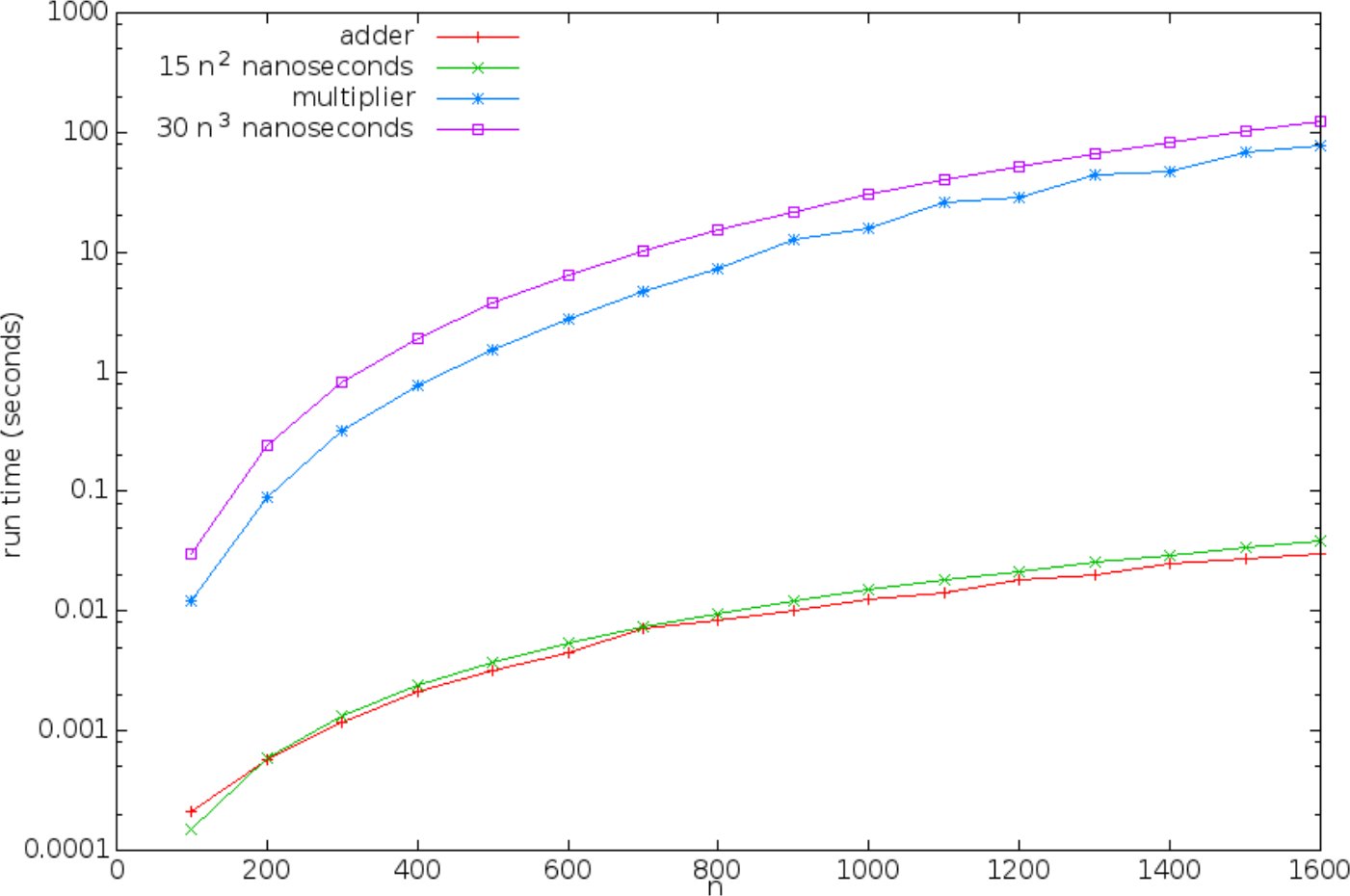
Profiling matrix operations run-time
Using measureCpuTimeRepeated, for matrix size \(n = 100, 200, \ldots, 1600\).
Fitting curves
- The previous running times were produced several years ago on a 3.1 GHz i5-2400 CPU with 8 GB RAM, and compiled using Scala 2.10.3.
- They are far outdated now.
- The exact running times will vary with computer system, but
The shape of the curves will stay the same!
Big-O notation
- Actual running times are more complex than the basic functions we just saw,
- E.g. \(f\left(n\right) = 150n^3 + 2n^2 + 3200\)
- or \(f\left(n\right) = 44 n \log n + 15n\)
- But, constants are often due to system or implementation specifics
- For large enough inputs the algorithm details tend to dominate
- The Big-O notation abstract away the constants and terms whose growth will be dominated by another term
Big-O notation
Definition (Big-O) ( "grows at most as fast as" ):
For two (positive, real-valued) functions,\(f\) and \(g\), defined over non-negative integers \(n\) we write \(f = \mathcal{O}(g)\) if there exist constants \(c,n_0 \gt 0\) such that \(f(n) \leq {c g(n)}\) for all \(n \geq n_0\).
- That is, \(f\) grows at most as \(g\) when \(n\) is large enough (up to a constant factor)
- We say that \(g\) is an asymptotic upper bound of \(f\)
- Note: Strictly speaking, use \(=\) in \(f = \mathcal{O}(g)\) is abuse of notation.
- The statement should be read as "\(f\) is \(\mathcal{O}(g)\)" and not as equality.
- (It does not make sense to say \(\mathcal{O}(g) = f\).)
- Formally, if we think of \(\mathcal{O}(g)\) as a set, then it is correct to say \(f \in \mathcal{O}(g)\).
'Common' functions
- Constant: \(c\), for some fixed constant
- Logarithmic: \(\log n\) (base usually 2)
- Linear: \(n\)
- Linearithmic or "n-log-n": \(n \log n\)
- Quadratic: \(n^2\)
- Cubic: \(n^3\)
- Polynomial: \(n^k\), for some fixed \(k > 0\) [generalisation of above]
- Exponential: \(d^n\), for some fixed \(d > 1\)
- Factorial: \(n!\)
Comparing scaling using \(\mathcal{O}\)
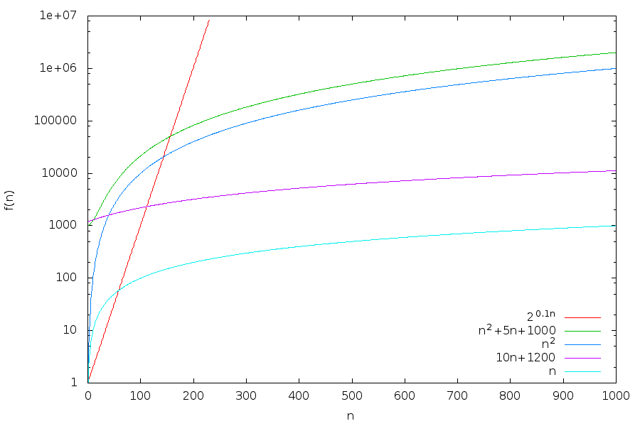
- \(n = \mathcal{O}\left(10n + 1200\right)\), by definition
- \(10n + 1200 = \mathcal{O}\left(n\right)\), because \(10n + 1200 \lt 12n\) when \(n > 600\)
- That is, \(10n + 1200\) and \(n\) are equivalent in the big-O notation
Comparing scaling using \(\mathcal{O}\)
- \(10n + 1200 = \mathcal{O}\left(n^2\right)\), because \(10n + 1200 \lt 10n^2\) when \(n > 12\)
- \(n^2 \neq \mathcal{O}\left(10n + 1200\right)\), because \(\lim \frac{n^2}{10n + 1200} \rightarrow \infty\) as \(n \rightarrow \infty\)
- \(n^2\) grows faster than \(10n + 1200\) in the big-O notation
Given the following definitions, is \(f_i = \mathcal{O}(f_j)\)?
- \(f_1(n) = n^2 + 5n + 1000\),
- \(f_2(n) = n^2 \),
- \(f_3(n) = 2^{0.5n}\),
- \(f_4(n) = 2^{\log n}\),
- \(f_5(n) = 18n\),
- \(f_6(n) = \log n\).
https://presemo.aalto.fi/prog2
Hint: Only degree matters for polynomial functions
\(\Omega\) and \(\Theta\)
We can also define an asymptotic lower bound (\(\Omega\)) and asymptotic equality (\(\Theta\)) for scaling as
Definition (\(\Omega\) - "grows at least as fast as" ):
\( f\left(n\right) = \Omega\left(g\left(n\right)\right)\), if and only if \(g\left(n\right) = \mathcal{O}\left(f\left(n\right)\right)\)
Definition (\(\Theta\) - "grows equally fast" ):
\(f\left(n\right) = \Theta\left(g\left(n\right)\right)\), if and only if \(f\left(n\right) = \mathcal{O}\left(g\left(n\right)\right)\) and \(f\left(n\right) = \Omega\left(g\left(n\right)\right)\)
Big-O for running times
The running time for a function/method/program is \(\mathcal{O}\left(f\right)\) if and only if for all inputs of size \(n\) the running time is \(\mathcal{O}\left(f\left(n\right)\right)\) time units.
- Big-O is an important concept in algorithms and CS theory
- Can be generalised to other resources as well, for example memory usage
- If you can prove that your algorithm is in \( \mathcal{O}\left(f\right) \) of some function \(f\) with respect to some resource (running time, memory, ..) you have put an asymptotic upper bound for how that resource requirement scales
- Therefore, when looking for \(\mathcal{O}\left( f \right)\) we are interested in an \(f\) that grows as slow as possible (while still obeying the definition of Big-O)
- Conversely, when determining \(\Omega\left(f\right)\), we want a function that grows as fast as possible
Analysis based on code - matrix multiplication
/** Returns a new matrix that is the product of this and that */
def *(that: Matrix): Matrix =
    val result = Matrix(n)
    for i <- 0 until n; j <- 0 until n do
        var v = 0.0
        for k <- 0 until n do
            v += this(i, k) * that(k, j)
        result(i, j) = v
    end for
    result
end *
We have to look at each statement and ask ourselves how many constant time instructions it takes.
Analysis based on code - matrix multiplication
/** Returns a new matrix that is the product of this and that */
def *(that: Matrix): Matrix =
    val result = Matrix(n)                      // O(n^2)
    for i <- 0 until n; j <- 0 until n do
        var v = 0.0
        for k <- 0 until n do
            v += this(i, k) * that(k, j)
        result(i, j) = v
    end for
    result
end *
A Matrix contains \(n^2\) numbers - each needs to be initialised.
Analysis based on code - matrix multiplication
/** Returns a new matrix that is the product of this and that */
def *(that: Matrix): Matrix =
    val result = Matrix(n)                      // O(n^2)
    for i <- 0 until n; j <- 0 until n do       // O(n^2)
        var v = 0.0
        for k <- 0 until n do
            v += this(i, k) * that(k, j)
        result(i, j) = v
    end for
    result
end *
The for loop goes through all \(n^2\) elements.
Analysis based on code - matrix multiplication
/** Returns a new matrix that is the product of this and that */
def *(that: Matrix): Matrix =
    val result = Matrix(n)                      // O(n^2)
    for i <- 0 until n; j <- 0 until n do       // O(n^2)
        var v = 0.0                             // O(n^2)
        for k <- 0 until n do
            v += this(i, k) * that(k, j)
        result(i, j) = v
    end for
    result
end *
Assignment is \(\mathcal{O}(1)\), but applied \(\mathcal{O}(n^2)\) times due to loop.
Analysis based on code - matrix multiplication
/** Returns a new matrix that is the product of this and that */
def *(that: Matrix): Matrix =
    val result = Matrix(n)                      // O(n^2)
    for i <- 0 until n; j <- 0 until n do       // O(n^2)
        var v = 0.0                             // O(n^2)
        for k <- 0 until n do                   // O(n^3)
            v += this(i, k) * that(k, j)
        result(i, j) = v
    end for
    result
end *
Loop by itself is \(\mathcal{O}(n)\), but inside \(\mathcal{O}(n^2)\) loop, so \(\mathcal{O}(n^3)\).
Analysis based on code - matrix multiplication
/** Returns a new matrix that is the product of this and that */
def *(that: Matrix): Matrix =
    val result = Matrix(n)                      // O(n^2)
    for i <- 0 until n; j <- 0 until n do       // O(n^2)
        var v = 0.0                             // O(n^2)
        for k <- 0 until n do                   // O(n^3)
            v += this(i, k) * that(k, j)        // O(n^3)
        result(i, j) = v
    end for
    result
end *
Several constant time operations inside loop. Important: Why are accessing values constant in this case?
Analysis based on code - matrix multiplication
/** Returns a new matrix that is the product of this and that */
def *(that: Matrix): Matrix =
    val result = Matrix(n)                      // O(n^2)
    for i <- 0 until n; j <- 0 until n do       // O(n^2)
        var v = 0.0                             // O(n^2)
        for k <- 0 until n do                   // O(n^3)
            v += this(i, k) * that(k, j)        // O(n^3)
        result(i, j) = v                        // O(n^2)
    end for
    result
end *
Performed \(\mathcal{O}(n^2)\) times. Again - assumes assignment of value to element is \(\mathcal{O}(1)\).
Analysis based on code - matrix multiplication
/** Returns a new matrix that is the product of this and that */
def *(that: Matrix): Matrix =
    val result = Matrix(n)                      // O(n^2)
    for i <- 0 until n; j <- 0 until n do       // O(n^2)
        var v = 0.0                             // O(n^2)
        for k <- 0 until n do                   // O(n^3)
            v += this(i, k) * that(k, j)        // O(n^3)
        result(i, j) = v                        // O(n^2)
    end for
    result                                      // O(1)
end *
Analysis of big-O based on code; rules of thumb
- Nested loops over the full problem (data) size will increase the order
- as everything inside the loop needs to be done \(n\) times.
- But note that loops can be dynamic (only accessing a subset)
- The same goes for recursion where we may want to be careful about how 'deep' the recursion goes
- (We will return to this later in this lecture)
- Method/function calls can hide complexity – know the efficiency of what you use
- Data structures matters!
- E.g. if we use Array or List to represent the matrix elements
- Therefore, always make sure you know what data structure is used
- Always document performance characteristics when you provide a library/package
- (Like Scala does for collections)
Matrix implementation if we had used a ListBuffer instead of an Array for the member value entries?)
Optimising the constant factor (i.e. optimising code)
- Big-O ignores constant factors; it is about the algorithm used
- Scaling of algorithms and data structures is extremely important for efficient programs
- But in practice, optimising for the constant factor can lead to further (large) savings in time (and energy)
- Example in the course notes optimising Matrix multiplication
- Results:
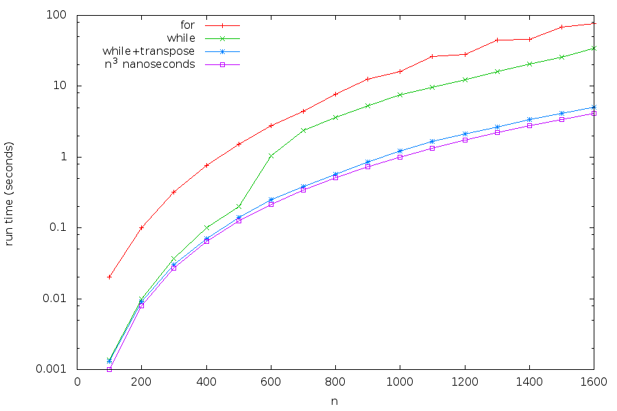
- | Using for--loops
- x Using while--loops
- * Using while--loops and matrix transpose
- □ \(n^3\) nanoseconds for reference
Almost 30-fold increase between for and while+transpose! (But still \(\mathcal{O}(n^3)\)…)
But, does efficiency matter?
- Yes!
- In practice, e.g
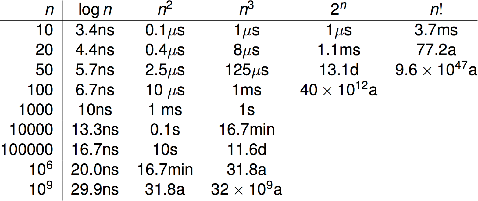
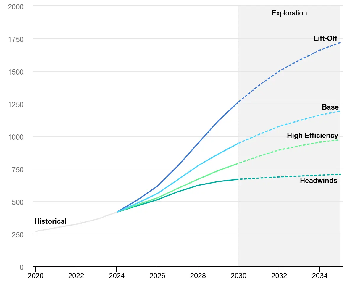
- huge data sets ⇒ huge \(n\)
- millions of users ⇒ app is run millions of times
- energy consumption* ⇐ computing generally require energy (Landauer's principle)
- In theory
- Computational complexity - the study of how hard problems are and what we fundamentally can compute
Searching - a common problem
- Finding an element in a collection is a very common problem
- Involves going over the elements in a collection until
- the element is found, or
- we know it isn't there
- As searching is very common the efficiency is important
Disorder and linear search
- If the collection is disordered (or we know nothing about it), then essentially the best we can do is Linear search
- E.g. Look for
19in(4,24,7,11,4,7,21,23,8,19,1,30) - Go through the collection start to finish until the element is found or we have reached the end
- E.g. Look for
def linearSearch[T](s: IndexedSeq[T], k: T): Boolean =
  var i = 0
  while(i < s.length)  do
    if(s(i) == k) then return true // found k at position i
    i = i + 1
  end while
  false // no k in sequence
end linearSearch
- Assuming testing for equality and indexed access (
s(i)) are constant time, linear search is \(\mathcal{O}(n)\). - Not bad, but very often code search the same collection many times repeatedly
- Say that we want to search for each element once ⇒ that code is \(\mathcal{O}(n^2)\)
- One
nfrom the repeated search times thenfrom the search itself
Indexing - imposing structure
- If we know that a collection will be searched repeatedly it could pay off to analyse it first
- This process is generally known as indexing
- The most common form of indexing is sorting
- (Requires that we have some idea about how to order the elements in some sense)
- Index is created once, so if that cost is not prohibitive, and it is effective to use this could pay off
Order and binary search
- Assume instead that we have a collection of perfectly ordered data
- E.g. look for
19in(1,4,4,7,7,8,11,19,21,23,24,30)
- E.g. look for
- Will this structure allow us to do better than linear search?
- Yes - binary search:
- Suppose we need to find the element
kin sequences - Assume
sis already sorted in ascending order - If
sis empty the element cannot be found. Stop. - Let
mbe the middle (rounded down) element ofs:- if
k=m, we are done. Stop. - if
k<m, then the key can only appear in the first half of the sequence- Recursively search over on the first half of
sonly
- Recursively search over on the first half of
- if
k>m, then the key can only appear in the second half of the sequence- Recursively search over on the second half of
sonly
- Recursively search over on the second half of
- if
- Suppose we need to find the element
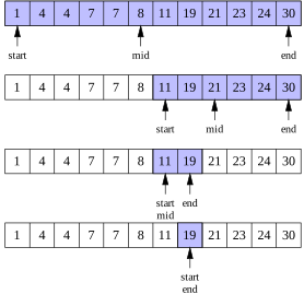
Binary search - example
- Suppose we need to find the element
kin sequences - Assume
sis already sorted in ascending order - If
sis empty the element cannot be found. Stop. - Let
mbe the middle (rounded down) element ofs:- if
k=m, we are done. Stop. - if
k<m, then the key can only appear in the first half of the sequence- Recursively search over on the first half of
sonly
- Recursively search over on the first half of
- if
k>m, then the key can only appear in the second half of the sequence- Recursively search over on the second half of
sonly
- Recursively search over on the second half of
- if
Binary search in Scala
def binarySearch[T](s: IndexedSeq[T], k: T)(using Ordering[T]) : Boolean =
  import math.Ordered.orderingToOrdered // To use the given Ordering
  //require(s.sliding(2).forall(p => p(0) <= p(1)), "s should be sorted")
  def inner(start: Int, end: Int): Int =
    if !(start < end) then start
    else
      val mid = (start + end) / 2
      val cmp = k compare s(mid)
      if cmp == 0 then mid                     // k == s(mid)
      else if cmp < 0 then inner(start, mid-1) // k < s(mid)
      else inner(mid+1, end)                   // k > s(mid)
    end if
  end inner
  if s.length == 0 then false
  else s(inner(0, s.length-1)) == k
end binarySearch
Efficiency of binary search
- Again, assuming comparisons (
=,<,>) and access takes constant time - Each 'step' of the binary search algorithm only contains \(\mathcal{O}(1)\) operations
- But, it is called recursively
- What is the maximum number of times it is called?
- Stops when element is found, or called on zero length sequence
- Each recursive call the length of the sequence is halved
- If the original sequence length is \(n\), then the recursive calls are of lengths \(\frac{n}{2^1},\frac{n}{2^2},\ldots\)
- until some \(\left\lfloor\frac{n}{2^k}\right\rfloor = 0\)
- That is in \(k = \log n\) recursive calls
- So binary search is \(\mathcal{O}(\log n)\)
Sorting + Binary search efficiency
- When the sequence is ordered search can be done in \(\mathcal{O}(\log n)\)
- Great, but what is the cost of sorting?
- Comparison-based sorting algorithms (Scala's
sortedmethod) work in time \(\mathcal{O}(n \log n)\)
- Comparison-based sorting algorithms (Scala's
- ⇒ efficiency of sort + search is \(\mathcal{O}(n \log n) + \mathcal{O}(\log n) = \mathcal{O}(n \log n)\)
- This is worse than linear search, \(\mathcal{O}(n)\)!
- Yes, but we only sort once!
- So, say you are doing \(n\) repeated searches, then effectively
- Binary search: \(\mathcal{O}(n \log n) + \mathcal{O}(n) \times \mathcal{O}(\log n) = \mathcal{O}(n \log n)\)
- Linear search: \(\mathcal{O}(n) \times \mathcal{O}(n) = \mathcal{O}(n^2)\)
- Rule of thumb: Only a handful of searches - it may not be worth processing the data, if the number of searches is large indexing pays off
Exercises
- Median and percentiles
- Quiz on Big-O
- Binary search: finding roots
- Binary search: finding subsets
- Pair sum
- Challenge: One terabyte
- Remember that Scala's
sortedmethod works in \(\mathcal{O}(n \log n)\) - Study the principle behind binary search and its Scala implementation in the course notes
- Draw a figure of the divide and conquer step in the binary search algorithms
- Play around with a few basic examples using pen and paper to develop an idea of how to do a fast pair sum