CS-A1120 Programming 2
  • Introduction
    • Round 1: Warmup
      • Sequences
        • Transforming sequences
      • Cascading
      • Recursion
      • Classes and objects
  • Module I: The mystery of the computer
    • Round 2: Bits and data
      • Introduction
        • Bits
        • Data
        • Data and its format
        • Types of data
        • Fixed-length data, words, word length
        • Variable-length data
        • Units of measure for data
        • Witnessing the bits, in Scala
        • Data and its format – a roadmap for this round
      • tellAboutX - Functions that expose the bits
      • Numerical data
        • The positional number system
        • Beyond base 10
        • Binary, octal, decimal, hexadecimal
        • Serendipity of hexadecimal
        • Bit positions in a word
        • Hexadecimal in Scala
        • Forcing and toggling bits in a word
        • Shifting the bits in a word
        • Four basic tricks of the trade
        • Packing and unpacking bits
        • Numerical computation (*)
        • Radix point notation (*)
        • Floating point numbers (*)
        • Arbitrary-precision numbers (**)
      • Textual data (*)
        • Representing individual characters (*)
        • Character encodings (*)
        • Strings (*)
        • Formatted text (*)
        • Tables as text (*)
        • Structured objects as text (*)
        • Programs as text – syntax and parsing (**)
        • Context-free grammars (**)
    • Round 3: Combinational logic
      • Introduction
        • Building machines that compute with bits, from the bottom up
        • Logic gates
        • The power of combination
        • Building combinational logic in Scala
        • Playing with a circuit
        • The art of bottom-up design – a roadmap for this round
      • Gate-level design
        • Defining operators in Scala
        • Our first design – the half adder
        • Specification and implementation – the truth table and synthesis
        • Configurability – data and control
        • Efficiency – circuit depth and size (*)
      • Bus-level design
        • Customizing Scala collections
        • Convention on indexing the bits in a bus
        • Functional design – encapsulating code that builds subcircuits
      • Arithmetic with words
        • Unsigned addition
        • The ripple-carry adder
        • Unsigned multiplication
        • Fixed-length arithmetic and overflows (*)
        • Signed integers (*)
      • Refresher: Objects, references, and recursion recalled
        • Objects and references recalled
        • Recursion recalled
    • Round 4: Sequential logic, state and feedback
      • Introduction
        • State, evolving the state
        • Feedback
        • Upgrade from tinylog to minilog
        • Our first design with sequential logic – the counter
        • Our second design – the accumulator-adder
        • Our third design – the accumulator-adder-subtracter
        • Towards understanding the computer
        • Building an instructable data path – a roadmap for this round
      • Sequential logic in Scala (*)
        • Designing with patterns (*)
        • Spotting common patterns in package tinylog (*)
        • Why tinylog needs upgrading (*)
        • Building feedback to an input element (*)
        • Implementing the clock signal functionality (*)
        • Registering all gates with a host (*)
        • Speeding up the simulation (*)
        • The art of designing with patterns (*)
      • The armlet data path
        • The armlet architecture overview
        • Registers and processor state
        • The arithmetic logic unit (ALU), first version
        • Extending the ALU – loading immediate data
        • Trigger time with the ALU
        • The ALU in Scala (**)
        • Memory and the armlet (*)
        • Memory interface unit
        • The load completion unit (*)
        • Summary
      • The armlet instruction set
        • An instruction – a symbol in the alphabet of the machine
        • Binary representation of the armlet instructions (**)
        • The instruction decoder unit
        • Instructing the data path with Trigger
        • Towards programmability
    • Round 5: A programmable computer
      • Introduction
        • Towards programmability
        • Storing the program in memory
        • Automating execution
        • Resolving the mystery of programmability – a roadmap for this round
      • The armlet processor
        • The data path
        • The program counter and processor status
        • The comparison instructions
        • Default flow of execution
        • The jump and branch instructions
        • Jumps and branches versus if-then-else, while, and such
        • Reset
        • Halt
        • Trap (debugging)
        • The armlet architecture (*)
      • Programming the armlet
        • Our first armlet program
        • Assembly language
        • The assembler
        • A playful introduction to Ticker
        • Beyond the first example
        • Scanning data
        • Sorting data
        • Some conventions and hints for the exercises
      • From Scala to hardware (*)
        • From Scala to bytecode for the Java Virtual Machine (*)
        • A second example (*)
        • Bytecode beyond our examples (**)
        • From bytecode to hardware (*)
      • Mystery resolved?
        • Software and hardware
        • The operating system (*)
        • Virtualization and simulation (*)
        • Programming environments (*)
        • Conclusion – it is important to understand hardware
  • Module II: Programming abstractions and analysis
    • Round 6: Collections and functions
      • Collections
        • Example: ArrayBuffer
        • Why so many collections?
      • Functions
        • Anonymous functions
        • Methods as functions
        • Side effects and pure functions
      • Using collections in functional style
        • forall
        • foreach
        • map
        • flatMap
        • groupBy
        • foldLeft
        • zip
        • indices and zipWithIndex
      • More on functions
        • Closure
        • Call-by-value and call-by-name
      • Iterators
        • Independent use: generators
    • Round 7: Efficiency
      • Resources and efficiency, with a focus on time
      • Measuring run time
      • Case: Operations on matrices
      • Growth rates of functions
        • Matrix operations revisited: Fitting a function
        • Typical functions
        • The Big O notation
      • Indexing and search
        • Disorder and order, searching
        • Linear search
        • Indexing and sorting
        • Binary search
    • Round 8: Recursion
      • Introduction
      • Recursion and tail recursion recalled
        • Example: Palindromes
        • Tail recursion
      • Linked lists
        • A first implementation
        • A second implementation with case classes
      • Expressions
        • Evaluation
        • Simplification
      • Solving problems recursively
        • The subset sum problem
        • A word on hard problems and NP-completeness
  • Module III: Frontiers
    • Round 9: Concurrency and parallelism
      • Introduction
        • A single thread of execution
        • Multiple threads
        • Why concurrency and multithreading?
        • Easy parallelism
      • Our first multithreaded program in Scala
        • Asynchronous execution
        • Synchronization
        • Why synchronization?
      • Independence and dependence
        • What can be computed in parallel?
        • A functional perspective
        • Independence
        • Dependence
        • Modelling dependence with directed acyclic graphs (DAGs)
        • Minimum makespan and scheduling
        • Parallel speedup and Amdahl’s law
        • What can be computed in parallel, revisited
      • Abstractions for easy parallelism
        • Futures and Promises
    • Round 10: Virtualization and scalability
      • Scaling up from a single computer
        • Computation becomes a commodity
      • Resiliency, partitioning, and dependence
        • What can be computed in a computer cluster?
        • Driver node and worker nodes
        • Hardware failures and resiliency
        • Partitioning and persistence (*)
      • Resilient distributed datasets
        • Transformations on RDDs
        • Actions on RDDs
        • Next step: Try it for yourself
      • An example of using Spark in Scala
        • Example context
        • The program
    • Round 11: Machines that learn?
      • Introduction
        • What is teaching? What is learning?
        • Generalisation from presented examples – a roadmap for this round
      • Generalisation beyond presented examples
        • Presented examples
        • Generalising into the unknown
        • The role of the programmer/teacher
        • Testing
      • Risks, rewards, and types of learning
        • Risks in learning
        • Serendipity of learning
        • Types of learning techniques
  • Appendix: Instructions
    • Using the Visual Studio Code editor
      • On Aalto Linux computers
      • Installation on personal computer
        • First things first
        • macOS
        • Linux
        • Windows 10 & 11
      • Setup
      • Workflow
      • Trouble-shooting
        • The Test and Run links don’t appear in my source code
        • Scala not found
        • Java not found
        • Error message about build server
        • sbt command not found
        • Error: code: No such file or directory (Aalto Linux workstation)
        • Error: the following module(s) are unknown (Aalto Linux workstation)
        • Warning: Code navigation will not work
    • Using the IntelliJ IDEA
      • Installing IntelliJ on your own computer
        • Fresh install
      • Installing the Scala language plugin
      • Working with the exercises
        • Running tests and code
        • Opening a Scala REPL
      • Trouble-shooting
        • scalac: Token not found:
    • Some basic tasks
      • Downloading exercise projects
      • Submitting your solutions for grading
      • Opening an sbt console from the command line
    • Getting help
      • On-campus exercise sessions
        • Queuing for help
      • On-line exercise sessions
      • Zulip workspace
        • Using
        • Etiquette
    • Accessing the Aalto VDI remote desktop
  • Acknowledgements
CS-A1120 Programming 2
  • »
  • Module II: Programming abstractions and analysis »
  • Round 7: Efficiency »
  • Indexing and search

Indexing and search

Everyday experience hints that if we get to choose between disorder and order, from the perspective of efficiency it may be serendipitous to choose order.

Indeed, look at the two sequences of characters below:

_images/unsorted-sorted.png

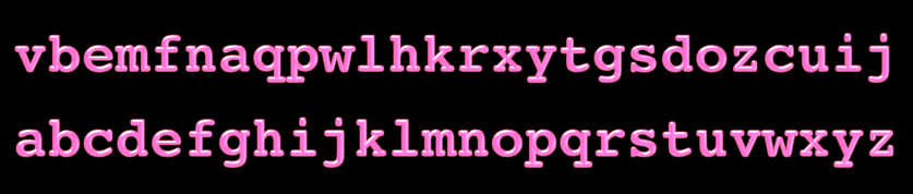
Both sequences contain the same characters.

The first sequence is arguably disordered (or unstructured), whereas the second sequence is arguably more ordered (or structured).

Disorder and order, searching

Suppose we now need to search a sequence of characters for a particular character, say, the character “x”:

  1. Does the character occur in the sequence?

  2. If so, how many times, and in what precise positions?

Again everyday experience suggests that order enables a more efficient search than disorder.

Let us, however, start with disorder.

Linear search

Suppose we are faced with an indexed sequence of elements of some type T. Suppose furthermore that we know absolutely nothing about the sequence. For all we know, there is no structure whatsoever in the sequence.

How efficiently can we search such a sequence for a particular element (or key) of type T ?

One possibility is just to perform a linear search, that is, we iterate through the sequence, one element at a time, and see whether we can find the key k:

def linearSearch[T](s: IndexedSeq[T], k: T): Boolean =
  var i = 0
  while(i < s.length)  do
    if(s(i) == k) then return true // found k at position i
    i = i + 1
  end while
  false // no k in sequence
end linearSearch

From the perspective of efficiency, if

  1. testing elements for equality, and

  2. indexed access to elements of the sequence

are both constant-time operations, then linear search takes \(\mathcal{O}(n)\) time for a sequence of length \(n\).

What is more, if we really know absolutely nothing about the sequence, then linear search is essentially the best we can do. That is, in the worst case we must access every element and test it for equality against the key k. Indeed, any element left unaccessed or untested could have been the only element that is equal to the key, so every element must be accessed and tested.

Note

The scala.collection classes that integrate the scala.collection.Seq trait use linear search to implement the method find through the scala.collection.Iterator trait

Warning

Despite its name, linear search may take more than linear time if it is not a constant-time operation to test two values of type T for equality. This is the case, for example, if the values are long strings or other complicated objects that may require substantial effort to test for equality.

Indexing and sorting

While linear search is the best we can do to search unstructured or unknown data, of course there is nothing that forces the data to remain unstructured once we have access to it.

Indeed, as soon as we have access, we should invest resources to introduce structure to the data to enable fast search. Once we know that the data has a particular structure, we can take advantage of this structure when we search the data.

Note

Such an approach of investing resources to introduce structure to enable subsequent fast search is called indexing the data.

Perhaps the most common form of indexing is that we sort the data so that the keys appear in increasing (or decreasing) order. Once we know that this is the case, then we can take advantage of the order when we search the data.

Binary search

Suppose we have a sequence \(s\) of elements that has been sorted to increasing order. Now suppose we must search whether a key \(k\) occurs in \(s\).

Consider the middle element \(m\) in \(s\). We observe the following three cases:

  1. If \(k = m\), we have found the key \(k\) so we can stop immediately.

  2. If \(k < m\), then the key \(k\) can appear only in the first half of the sequence.

  3. If \(k > m\), then the key \(k\) can appear only in the second half of the sequence.

In the latter two cases, we recursively continue in the selected half of the sequence until either

  • we find the key \(k\), or

  • the subsequence under consideration is empty, in which case we conclude that the key \(k\) does not appear in \(s\).

For example, below we display the steps of binary search for the key 19 in the ordered sequence [1,4,4,7,7,8,11,19,21,23,24,30]. In each step, we highlight with blue the current subsequence defined by the indices start and end:

_images/binarySearch.svg

That is, in the first step we start with the entire sequence and consider its middle element 8 (let us agree that when the sequence has even length, the middle element is the leftmost of the two available choices for the middle element). As the sequence is sorted and 8 is less than the key 19, we conclude that 19 can occur only in the second half of the sequence, not including the middle element 8. We then repeat the same with the subsequence consisting of the second half. Its middle element is 21, which is greater than the key 19. We thus next consider the first half of this subsequence, whose middle element is 11. In the last step the subsequence consists of one element, and this element is both the middle element and is equal to the key 19. Thus we have discovered 19 in the sequence. Observe that only the 4 elements (8, 21, 11 and 19) indexed by the middle point index mid in the figure are compared against the key 19.

As a second example, let us search for the key 6 in the same sorted sequence:

_images/binarySearch2.svg

In the last step, there are no more elements to consider in the subsequence and we conclude that 6 does not appear in the sequence.

Implementing binary search in Scala

Now that we understand how binary search operates, let us implement it in Scala.

First, we must make sure that our sequence is sorted and supports constant-time indexed access to its elements. If this is not the case, we prepare a sorted copy of the sequence with the sorted method and then (if necessary) transform the sorted collection into a type that supports constant-time indexed access, for example, by calling its toIndexedSeq (or toArray or toVector) method.

As we are not modifying the sequence during search, we need not create new sequence objects for the considered subsequences but can simply track the start and end of the current subsequence with two indices (start and end).

We can now implement binary search as a recursive function:

def binarySearch[T](s: IndexedSeq[T], k: T)(using Ordering[T]) : Boolean =
  import math.Ordered.orderingToOrdered // To use the given Ordering
  //require(s.sliding(2).forall(p => p(0) <= p(1)), "s should be sorted")
  def inner(start: Int, end: Int): Int =
    if !(start < end) then start
    else
      val mid = (start + end) / 2
      val cmp = k compare s(mid)
      if cmp == 0 then mid                     // k == s(mid)
      else if cmp < 0 then inner(start, mid-1) // k < s(mid)
      else inner(mid+1, end)                   // k > s(mid)
    end if
  end inner
  if s.length == 0 then false
  else s(inner(0, s.length-1)) == k
end binarySearch

Let us test the function with some sample inputs:

scala> val s = Vector(1,4,4,7,7,8,11,19,21,23,24,30)
s: scala.collection.immutable.Vector[Int] = Vector(1, 4, 4, 7, 7, 8, 11, 19, 21, 23, 24, 30)

scala> binarySearch(s, 19)
res: Boolean = true

scala> binarySearch(s, 6)
res: Boolean = false

Observe that the recursion takes place in the inner function inner because the recursive calls have to know the start and end of the current subsequence, and these parameters are not available in the outer function binarySearch. Also, the first require statement is not included but rather is commented out because its evaluation is (for long sequences) substantially slower than the rest of the function. One can include it, for instance, in the testing phase of a larger project so that illegal calls to the function with non-sorted sequences can be caught.

For a sorted sequence with \(n\) elements with constant-time indexed access and compare operator, the run-time of binarySearch is in \(\mathcal{O}(\log n)\):

  • The number of elements under consideration, end - start + 1, at least halves in each recursive call

  • We stop when start >= end (that is, when end - start + 1 <= 1)

  • How many halvings suffice until we have decreased the original \(n\)-element sequence into a one-element sequence? Denoting the number of halvings by \(h\), we have \(n/2^h \le 1\), which implies \(n \le 2^h\) and thus \(h \ge \log n\).

  • Under the previous assumptions, each halving takes constant time and thus the run-time is \(\mathcal{O}(\log n)\).

The number of calls to the compare operator is \(\mathcal{O}(\log n)\). This matters in particular if comparison is an expensive operation, for example, when the elements are long strings or other more complicated objects.

We have thus established that compared with linear search, binary search is a very fast way to search for a key in a sorted sequence.

If the sequence is initially not sorted but we have to sort it first to enable binary search, then we should include the time to sort into the analysis. The most efficient general purpose comparison-based sorting algorithms, such as the sorting algorithm that is implemented in the sorted method, work in time \(\mathcal{O}(n \log n)\). (Here we again assume comparisons are constant-time operations.) Now, if the sequence is initially unstructured and we make only one search after the sequence is sorted, the total run-time will be \(\mathcal{O}(n \log n) + \mathcal{O}(\log n) = \mathcal{O}(n \log n)\), which is in total slower than just running linear search on the unstructured input without sorting. On the other hand, if we make a large number of searches to the sequence then it pays off to first sort and then run binary search. Similarly, if we can afford to invest time to preprocess our input before any searches take place, and each search needs to be executed as fast as possible (for example, to supply a smooth and responsive user experience), then it again pays off to use binary search.

Note

Although binary search is conceptually quite straightforward, its implementations are surprisingly prone to subtle errors.

Note

The declaration implicit ev: T=>Ordered[T] in the function says that the class T of the elements in the sequence s must be such that it can be converted to an Ordered[T] class which provides the compare method used in the function. Moreover that a function ev (evidence) should be provided implicitly by Scala if such a conversion exists, so that the function can be called as binarySearch(s,k).

Note

Recursion is a natural way to implement binary search but we can also make an iterative implementation:

def binarySearchIter[T](s: IndexedSeq[T], k: T)(using Ordering[T]): Boolean =
  import math.Ordered.orderingToOrdered // To use the given Ordering
  //require(s.sliding(2).forall(p => p(0) <= p(1)), "s should be sorted")
  if s.length == 0 then return false
  var start = 0
  var end = s.length - 1
  while(start < end) do
    val mid = (start + end) / 2
    val cmp = k compare s(mid)
    if cmp == 0 then {start = mid; end = mid}
    else if cmp < 0 then end = mid-1  // k < s(mid)
    else start = mid+1                // k > s(mid)
  end while
  return s(start) == k
end binarySearchIter
Previous Next

© Copyright 2013-2022, Petteri Kaski, Tommi Junttila, and Lukas Ahrenberg.

Built with Sphinx using a theme provided by Read the Docs.