Growth rates of functions
As we observed with the two case studies, the run time of functions/algorithms/programs can be measured as a function of the size of the input (or some other natural parameter of the input).
What is fundamental in such studies is typically not the exact run time but rather the scalability or the rate of growth of the function that captures the running time. Indeed, it is often rather difficult (if not outright impossible) to exactly describe the run time of an algorithm in a manner that is reproducible beyond the exact hardware and software configuration and the exact computer load that was used in the measurements.
In what follows we proceed to make more precise in a mathematical setting what we mean by rate of growth and scalability to make meaningful analyses and comparisons possible.
Matrix operations revisited: Fitting a function
Let us revisit our case study with matrices, starting with the method for matrix addition.
    /* Returns a new matrix that is the sum of this and that */
    def +(that: Matrix): Matrix =
      val result = new Matrix(n)
      for row <- 0 until n; column <- 0 until n do
        result(row, column) = this(row, column) + that(row, column)
      result
    end +
Our intent is to describe the run time of this method as accurately as possible as a function of the dimension \(n\) of the matrix. Intuitively this should be a relatively straightforward task since the method has rather simple structure.
To perform a rough analysis, let us review what the method does and introduce some formal variables \(t_x\) for elementary operations that we witness as we proceed with the review.
To start with, we observe that the method first allocates a new
matrix, result. This operation involves allocation memory for
the new Matrix object itself and also for the \(n \times n\) entries
in the matrix, taking time \(t_{i,1}\) (\(i\) meaning ‘initialization’) . The \(n^2\) entries in the array are
also (implicitly) initialized to 0.0.
Thus, this initialization phase takes roughly
\(t_{i,1} + n^2 t_{i,2}\) time, where \(t_{i,2}\) is the time
taken to initialize one entry in the array.
Next, the method executes the for-loop.
The variable row is increased \(n\) times, each increase taking
some time \(t_{l,1}\). The variable column is increased \(n \times n\) times,
each taking time \(t_{l,2}\). The body of the loop is executed
\(n \times n\) times, each iteration taking \(t_{l,3}\) time.
The loop in total thus takes roughly time
\(n t_{l,1} + n^2(t_{l,2} + t_{l,3})\).
Finally, the algorithm returns the result, taking time \(t_{e}\). Thus the total time is rouhgly \(t_{i,1} + n^2 t_{i,2} +n t_{l,1} + n^2 (t_{l,2} + t_{l,3}) + t_{e}\).
So far so good, we have a formula that roughly reflects how much time (how many elementary operations) it takes to execute the method, as a function of the parameter \(n\).
Of course we do not yet have any concrete values for the formal time variables \(t_x\) that we introduced during our analysis. These values in general depend on a rather large number of factors, including
the clock speeds of the hardware (CPU and memory) on which we are executing the code,
the precise microarchitectural and configuration details of the hardware,
the level of optimization of the byte code compiled from our Scala source code (i.e., how good is the scala compiler that we used), and
the level of optimization of the byte code interpreter (the Java Virtual Machine) we are using.
Looking at this list, it looks like a formidable task to try to obtain precise values for the variables \(t_x\). Thus, instead of pursuing a precise answer, let us try to develop a rough answer.
Towards this end, perhaps it is a fair guess that the memory allocation as well as the time spent in returning the result are negligible when compared with the other parts of the method. Furthermore, for a matrix of dimension \(n\), with \(n\) large enough, it looks like the the initialization of the matrix entries and the for-loop body are the most executed parts of the method, each is executed \(n \times n\) times, so it would appear like a fair guess that this is the part of the method where most time is spent. So let us abstract the run time as \(c_1 n^2\), where \(c_1\) is some constant. (The big O notation that we will introduce in what follows will give a more formal theoretical justification why this kind of rough simplification makes sense if we are interested in scalability.)
Before we proceed to the big O notation, let us still consider another example. Namely, us do a similar analysis for the multiplication code.
    /* Returns a new matrix that is the product of this and that */
    def *(that: Matrix): Matrix =
      val result = new Matrix(n)
      for row <- 0 until n; column <- 0 until n do
        var v = 0.0
        for i <- 0 until n do
          v += this(row, i) * that(i, column)
        result(row, column) = v
      end for
      result
    end *
Here we observe that the innermost part of the loops, namely
the statement v += this(row, i) * that(i, column), is executed \(n^3\) times,
whereas all other parts are executed only \(n^2\) times at most. Thus
it would appear like a fair guess that we could roughly approximate
the run time of the method as \(c_2 n^3\), where \(c_2\) is again some constant.
To validate this approach empirically before proceeding any further, let us see how well the rough approximations meet reality. That is, let us choose values for the constants \(c_1\) and \(c_2\), and see how well our approximations \(c_1n^2\) and \(c_2n^3\) perform in relation to actual run times on inputs of dimension \(n\).
Let us make a rough guess that \(c_1\) is \(15\) nanoseconds and that \(c_2\) is \(30\) nanoseconds in the particular hardware + software configuration on which we run the tests. Plotting these approximations together with the actual empirical run times, we get:
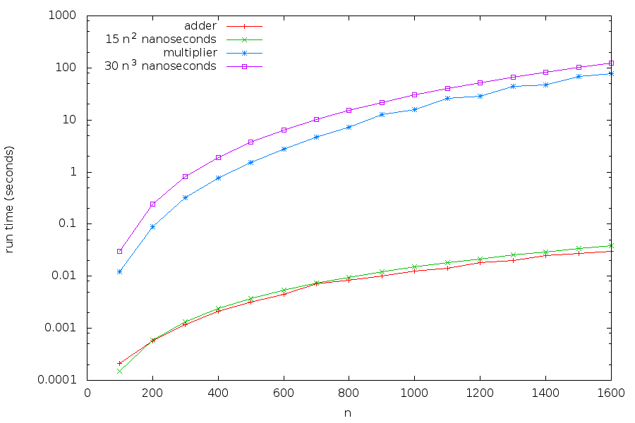
Our rough approximations appear to be not bad at all!
Typical functions
To obtain a light start to a more mathematical analysis, let us make an inventory of a few functions that are recurrently encountered when analysing scalability:
Constant: \(c\) for some fixed constant \(c\)
Logarithmic: \(\log n\) (usually the base is assumed to be \(2\))
Linear: \(n\)
Linearithmic or “n-log-n”: \(n \log n\)
Quadratic: \(n^2\)
Cubic: \(n^3\)
Polynomial: \(n^k\) for some fixed \(k > 0\)
Exponential: \(d^n\) for some fixed \(d > 1\)
Factorial: \(n!\)
We will see examples of algorithms whose run times belong to these classes in a moment but let us first compare the behaviour of the functions as such. How fast do these functions grow when we increase \(n\) ?
Let us take the functions \(1\), \(\log n\), \(n\), \(n \log n\), \(n^2\), \(n^3\), \(2^n\) and \(n!\). Plotting these functions with a linear \(y\)-axis, we observe:
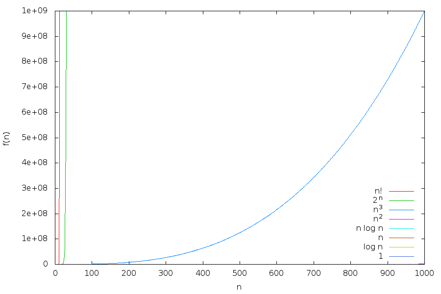
It looks like that the functions \(n!\) and \(2^n\) grow so fast that the other functions are rather dwarfed in comparison. So let us switch to logarithmic scale for the \(y\)-axis:
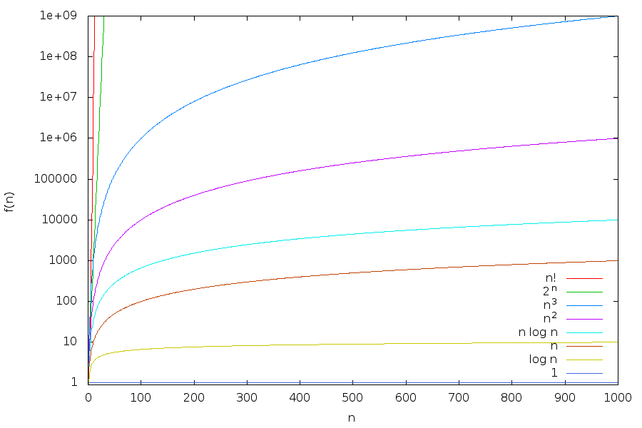
From the plots we can observe, for example, that
the logarithm \(\log n\) grows very slowly. For instance, \(\log 10^9 \approx 30\), and we can consider \(\log n\) almost as a constant function and \(n \log n\) almost as a linear function,
low-degree polynomials such as \(n\) and \(n^2\) still grow quite slowly, and
\(2^n\) and especially \(n!\) explode off the chart very quickly.
Let us study the same functions in tabular form:
\(n\) |
\(\log n\) |
\(n^2\) |
\(n^3\) |
\(2^n\) |
\(n!\) |
|---|---|---|---|---|---|
\(10\) |
\(3.33\) |
\(100\) |
\(1000\) |
\(1024\) |
\(3628800\) |
\(20\) |
\(4.33\) |
\(400\) |
\(8000\) |
\(1048576\) |
\(2.5\times10^{18}\) |
\(50\) |
\(5.65\) |
\(2500\) |
\(125000\) |
\(1.2\times10^{15}\) |
\(3.1\times10^{64}\) |
\(100\) |
\(6.65\) |
\(10000\) |
\(10^6\) |
\(1.3\times10^{30}\) |
|
\(1000\) |
\(9.97\) |
\(10^6\) |
\(10^9\) |
||
\(10000\) |
\(13.3\) |
\(10^8\) |
\(10^{12}\) |
||
\(100000\) |
\(16.7\) |
\(10^{10}\) |
\(10^{15}\) |
||
\(10^6\) |
\(20.0\) |
\(10^{12}\) |
\(10^{18}\) |
||
\(10^9\) |
\(29.9\) |
\(10^{18}\) |
\(10^{27}\) |
To get perspective on the large numbers in the table, let us assume that \(1\) unit corresponds to \(1\) nanosecond (\(10^{-9}\) seconds, or about \(3\) clock cycles in a modern CPU running at \(3\) GHz). Then the above table looks like this:
\(n\) |
\(\log n\) |
\(n^2\) |
\(n^3\) |
\(2^n\) |
\(n!\) |
|---|---|---|---|---|---|
\(10\) |
3.4 nanoseconds |
0.1 microseconds |
1 microsecond |
1 microsecond |
3.7 milliseconds |
\(20\) |
4.4 nanoseconds |
0.4 microseconds |
8 microseconds |
1.1 milliseconds |
77.2 years |
\(50\) |
5.7 nanoseconds |
2.5 microseconds |
125 microseconds |
13.1 days |
\(9.6\times10^{47}\) years |
\(100\) |
6.7 nanoseconds |
10 microseconds |
1 milliseconds |
\(40\times10^{12}\) years |
|
\(1000\) |
10 nanoseconds |
1 millisecond |
1 second |
||
\(10000\) |
13.3 nanoseconds |
0.1 seconds |
16.7 minutes |
||
\(100000\) |
16.7 nanoseconds |
10 seconds |
11.6 days |
||
\(10^6\) |
20.0 nanoseconds |
16.7 minutes |
31.8 years |
||
\(10^9\) |
29.9 nanoseconds |
31.8 years |
32 billion years |
Concerning growth rates, two further illustrative observations are as follows:
If the runtime of an algorithm is \(n^2\) and we can solve problems with input size \(n\) in time \(t\), then obtaining a machine that runs twice as fast enables us to solve problems with input size \(\sqrt{2}n\) in the same time \(t\).
If the runtime of an algorithm is \(2^n\) and we can solve problems with input size \(n\) in time \(t\), then obtaining a machine that runs twice as fast enables us to solve problems with input size \(n+1\) in the same time \(t\).
More generally, with polynomial \(n^k\) scaling, a machine twice as fast enables us to consider a constant (\(2^{1/k}\)) times larger inputs in the same time. With exponential \(d^n\) scaling, a machine twice as fast enables us to consider inputs that are larger by an additive constant (\(\log 2/\log d\)).
Exponential growth thus is rather explosive compared with polynomial growth.
The Big O notation
As we have witnessed so far, the run time of functions/algorithms/programs can be viewed as a function of the size of the input (or some other natural parameter), but exact analysis of such functions is rather involved.
We now introduce the standard mathematical tool for expressing and comparing rates of growth of functions: the big O notation. This notation concentrates on scalability by abstracting away
small instances (small sizes), and
multiplicative constants caused by factors that affect the run-time some constant amount, for example, CPU clock speed, pipeline efficiency, memory bandwidth, and so forth.
Our focus remains on run time, even if the big O notation can be used to analyse scalability in terms of consumption of other resources as well.
Let \(f\) and \(g\) be some functions from non-negative integers to non-negative reals (or rationals or integers). We say that “\(f\) is \(\mathcal{O}(g)\)”, or “\(f\) grows at most as fast as \(g\)”, if for large enough values of \(n\) (that is, large enough inputs) the value \(f(n)\) is at most \(c g(n)\) for some fixed constant \(c\geq 0\).
Formally:
Definition: \(\mathcal{O}\) (big O)
For two positive, real-valued functions \(f\) and \(g\) defined over non-negative integers \(n\) we write \(f(n) = \mathcal{O}(g(n))\) if there exist constants \(c,n_0 \gt 0\) such that \(f(n) \leq {c g(n)}\) for all \(n \geq n_0\).
Here the requirement “for all \(n \ge n_0\)” abstracts away small sizes and “\(f(n) \le {c g(n)}\)” the multiplicative constant factors such as CPU clock speed when talking about time efficiency.
In other words, if \(f(n) = \mathcal{O}(g(n))\), then \(g\) is an upper bound for the growth rate of \(f\). (For large enough instances and ignoring multiplicative factors.)
Strictly speaking, the use of \(=\) in the definitions of this chapter is not formally correct, and abuses the mathematical notation somewhat. You should read the operator as “is” rather than “equals”. If one sees \(\mathcal{O}(g(n))\) as a set of functions, then writing \(f(n) \in \mathcal{O}(g(n))\) would be more precise.
\(100n^2+n+50 = \mathcal{O}(n^2)\) because \(100n^2+n+50 \le 101n^2\) for all \(n \ge 8\). That is, for “large enough” instances, \(100n^2+n+50\) is at most a constant factor slower than \(n^2\), and thus we can see \(n^2\) as an upper bound for the growth rate of \(100n^2+n+50\). Of course we also have \(n^2 = \mathcal{O}(100n^2+n+50)\) as well.
Example
Now let us compare different functions under the big O notation. Take the functions \(n\), \(10n+1200\), \(n^2\), \(n^2+5n+1000\) and \(2^{0.1n}\). When plotted, the functions look like this:
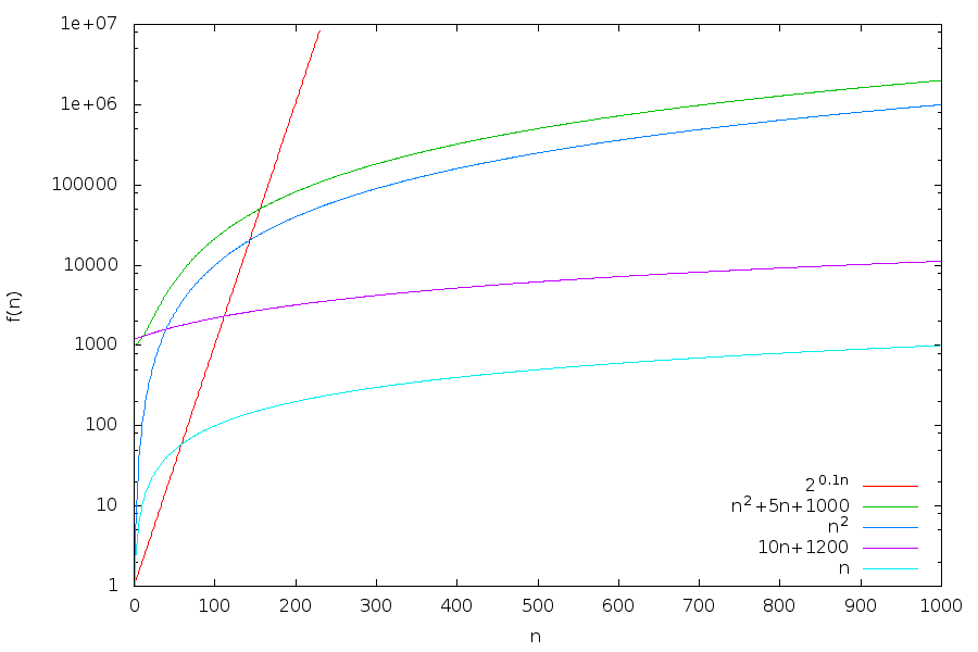
Let us analyse what we see in the above plot:
Compare \(n\) and \(10n+1200\). After the big gap for smallish values of \(n\), the distance between the plots in the log-scale seems to approach a constant, meaning that \(10n+1200\) is roughly only a constant times larger than \(n\). Indeed, already at \(500\) we have \(\frac{10\times500+1200}{500} = 12\) and \(\lim_{n\to\infty}\frac{10n+1200}{n} = 10\). These functions are the same also under big O notation:
\(10n + 1200 = \mathcal{O}(n)\) because \(10n + 1200 \le 12n\) for all \(n \ge 500\), and
\(n = \mathcal{O}(10n+1200)\) trivially.
Therefore, when we compare the growth rates of \(10n+1200\) and \(n\), we can use \(n\) as an approximation. (Indeed, \(n\) is the intuitively simpler function.)
The same happens when we compare \(n^2\) and \(n^2+5n+1000\).
When we compare \(n\) and \(n^2\), we see that the gap between them seems to grow steadily. And in fact it holds that \(\lim_{n\to\infty}\frac{n^2}{n} = \infty\). Thus \(n^2\) grows faster than \(n\). Or slightly more generally, quadratic functions grow faster than linear functions. And more generally, when considering growth rates of polynomial functions, only the degree of the polynomial matters.
Comparing \(n^2\) and \(2^{0.1n}\) graphically, we see that for small values of \(n\) the function \(n^2\) is considerably larger. But after the value \(144\), the function \(2^{0.1n}\) grows much faster. Analytically, we can see that \(\frac{2^{0.1n}}{n^2}\) grows without bound by observing \(\lim_{n \to \infty}\log\frac{2^{0.1n}}{n^2} = \lim_{n \to \infty}(0.1n - 2\log n) = \infty\) (if the logarithm of \(n\) goes to infinity, then so does \(n\)). Thus \(2^{0.1n} \neq \mathcal{O}(n^2)\). But \(n^2 = \mathcal{O}(2^{0.1n})\) as \(\lim_{n \to \infty}\log\frac{n^2}{2^{0.1n}} = \lim_{n \to \infty}(2\log n - 0.1n) = -\infty\) (if the logarithm of \(n\) approaches negative infinity, then \(n\) approaches zero). In general, exponential functions grow faster than any polynomial function.
The big O classification of functions is transitive, that is, if \(g\) is an upper bound for \(f\) and \(h\) is an upper bound for \(g\), then \(h\) is an upper bound for \(f\):
Lemma: Transitivity of \(\mathcal{O}\).
If \(f(n) = \mathcal{O}(g(n))\) and \(g(n) = \mathcal{O}(h(n))\), then \(f(n) = \mathcal{O}(h(n))\).
Proof:
If \(f(n) = \mathcal{O}(g(n))\), then there are constants \(c,n_0 \ge 0\) such that \(f(n) \le {c g(n)}\) for all \(n \ge n_0\). Similarly, if \(g(n) = \mathcal{O}(h(n))\), then there are constants \(d,m_0 \ge 0\) such that \(g(n) \le {d h(n)}\) for all \(n \ge m_0\). Thus \(f(n) \le c g(n) \le c(d h(n))\) for all \(p \ge \max(n_0,m_0)\).
One can also consider the dual of big O (big-Omega, a lower bound) and their combination (big-Theta, an “exact” bound):
Definition: \(\Omega\) (big-Omega) and \(\Theta\) (big-Theta)
We write \(f(n) = \Omega(g(n))\) if there exist constants \(c,n_0 \gt 0\) such that \(f(n) \ge {c g(n)}\) for all \(n \ge n_0\).
We write \(f(n) = \Theta(g(n))\) if both \(f(n) = \mathcal{O}(g(n))\) and \(f(n) = \Omega(g(n))\).
The relation between big O and big-Omega is as expected: \(g\) is an upper bound for \(f\) if and only if \(f\) is a lower bound for \(g\).
Lemma
If \(f(n) = \mathcal{O}(g(n))\), then \(g(n) = \Omega(f(n))\). Similarly, if \(f(n) = \Omega(g(n))\), then \(g(n) = \mathcal{O}(f(n))\).
Proof:
If \(f(n) = \mathcal{O}(g(n))\), then there are constants \(c,n_0 \ge 0\) such that \(f(n) \le {c g(n)}\) for all \(n \ge n_0\). Thus \(g(n) \ge \frac{1}{c}f(n)\) for all \(n \ge n_0\), implying that \(g(n) = \Omega(f(n))\). The proof of the second claim is analogous.
For example, we have seen above that
\(n^2+5n+1000 = \Theta(n^2)\),
\(2^{0.1n} = \Omega(n^2)\), and
\(n^2 = \Omega(n)\).
Observe that for exponential functions even small increases in the exponent do matter. For instance, compare \(2^{0.1n}\) and \(2^{n}\) Obviously, \(2^{0.1n} = \mathcal{O}(2^{n})\) as \(2^{0.1n} \le 2^{n}\) for all \(n \ge 1\). But \(2^{n} \neq \mathcal{O}(2^{0.1n})\) as the ratio \(\frac{2^{n}}{2^{0.1n}} = 2^{0.9n}\) grows without bound as \(n\) increases.
Examples
Let us now review some examples of typical run times in big O notation.
Constant time \(\mathcal{O}(1)\): Primitive arithmetic operations.
Primitive operations, such as addition, multiplication, Boolean operations, and so forth, take constant time on the primitive types like Boolean, Int, and Double. For instance, if
xandyare Doubles, thenx + yandx * ycan be computed in constant amount of time.But observe that
x + yandx * yare not constant time operations wheneverxand/oryare of type BigInt. BigInts allow arbitrary large numbers and, for instance, adding two \(n\) bit numbers must take at least \(\mathcal{O}(n)\) time. As Scala (and many other modern programming languages) allow operator overloading, one has to be a bit carefull when reading code: innocent looking operators (like*above) may lead to time-consuming computations.Constant time \(\mathcal{O}(1)\): Random access to arrays.
Accessing the element at position \(i\) in an Array object
arrusingarr(i)is a constant-time operation because arrays are natively supported by the underlying virtual machine and hardware, which also has constant time access to array.In contrast, if we have a List object
l, thenl(i)is not a constant time operation: the lists are implemented in a way that requires, in the worst case, \(\mathcal{O}(n)\) elements to be traversed in a list of length \(n\). We will study lists in more detail later.Note
Time requirements of access and update operations for typical collection data types.
As we already know, the different basic collection data types in the scala.collection package have differing internal implementations and thus differing performance characteristics. The most important operations and their time requirements can be found ìn this table. For now, you can read “effectively constant time” and “amortized constant time” simply as “constant time”, a more detailed study of data structures and their operation will be conducted in the course CS-A1140 Data Structures and Algorithms.
Linear time \(\mathcal{O}(n)\): Finding an element in disordered data.
Suppose that we have an Array
arrof \(n\) integers and that the integers in the array are completely disordered. Then finding whether a specific integerxoccurs in the array with, for example,arr.contains(x)takes \(\mathcal{O}(n)\) time: in the worst casexis not in the array and and we have to compare all the \(n\) integers in the array toxto deduce this fact, where each comparison takes constant time \(\mathcal{O}(1)\). In the best case the integerxis the first element in the array. Thus the lower bound for the run time is \(\Omega(1)\).The situation changes if the integers in the array are ordered (sorted) (see this section).
Quadratic time \(\mathcal{O}(n^2)\): Insertion sorting.
Assume that we have an array of integers and we want to sort them to increasing order. For instance, we wish to transform
Array(4, -3, 3, 2, 1, -2)intoArray(-3, -2, 1, 2, 3, 4). An algorithm performing this task is called a sorting algorithm.One of the simplest sorting algorithms is the insertion sort algorithm, which relies on the following idea: for each position \(i=0,1,2,\ldots,n-1\) in the array, the algorithm looks at the element \(x\) in position \(i\) and moves \(x\) towards the beginning of the array as long as \(x\) is smaller than the element just before it (if any). In particular, after considering position \(i\), the sub-array consisting of the first \(i+1\) elements is in sorted order, and hence the entire array is in sorted order after \(i=n-1\) has been considered. (An animation illustrating the algorithm is available here.) In Scala, we can implement insertion sort as follows:
def insertionSort(a: Array[Int]) =
  for(i <- 0 until a.length) do
    val x = a(i)
    var j = i
    while(j > 0 && x < a(j-1)) do
      a(j) = a(j-1)
      j = j - 1
    end while
    a(j) = x
  end for
end insertionSort
At the console we observe:
scala> val a = Array(4,-3,3,2,1,-2)
a: Array[Int] = Array(4, -3, 3, 2, 1, -2)
scala> insertionSort(a)
scala> a
res: Array[Int] = Array(-3, -2, 1, 2, 3, 4)
Let us now analyse the algorithm. If we have an array of \(n\) integers, then the
forloop is executed \(n\) times. At iteration \(i\), thewhileloop is executed at most \(i\) times. All the other operations use constant time. Thus, the total run time is \(\mathcal{O}(\frac{n(n-1)}{2}) = \mathcal{O}(n^2)\).The best-case performance occurs when the array is already sorted: at each iteration of the
forloop, the body of thewhileloop is executed at most once, which leads to an \(\Omega(n)\) lower bound for the run time.Many different sorting algorithms with differing characteristics exist. In Scala, the mentod
sortedinSeqrelies on the sort functionality in Java’sArrayclass, which implements a sorting algorithm with \(\mathcal{O}(n \log n)\) running time (subject to the assumption that the task of comparing two elements take constant time).Cubic time \(\mathcal{O}(n^3)\): Matrix multiplication.
We have already seen in the sub-section Matrix operations revisited: Fitting a function that multiplying two \(n\)-by-\(n\) matrices can be done in time \(\mathcal{O}(n^3)\), where \(n\) is the dimension of the matrix (not the amount of space taken by the matrix, which is \(\mathcal{O}(n^2)\)). As our example algorithm for doing this does not contain any conditions, its best case performance is the same as the worst case, meaning that its run time is \(\Omega(n^3)\) and thus \(\Theta(n^3)\).
Remark. Faster algorithms for multiplying two matrices are known, for example Strassen’s algorithm and Le Gall’s algorithm.
Exponential time: Iterative squaring with arbitrary precision.
Consider the following code:
def f(n:Int): BigInt =
  require(n >= 0)
  var result: BigInt = 2
  for(i <- 0 until n) do result = result * result
  result
end f
The call
f(n)computes the number \(2^{2^n}\), whose binary presentation requires \(2^n\) bits. Even though the code has a loop consisting of only \(n\) iterations, its run time is \(\Omega(2^n)\) because the line “result = result * result” doubles the length of the binary representation ofresulteach time it is executed, and multiplying two \(i\)-bit numbers takes time \(\Omega(i)\).Factorial time: Iterating through all permutations.
Recall that a permutation of a set of objects is an arrangement of those objects in some order. For instance, if we have the objects “a”, “b”, and “c”, then (“a”,”b”,”c”) and (“c”,”b”,”a”) are two permutations of the objects. In general, if we have a set of \(n\) distinct objects, then there are \(n!\) (”\(n\) factorial”) distinct permutations of the objects. In Scala, the sub-classes of the sequence trait Seq, such as List and ArrayBuffer, have the method
permutationsthat allows us to iterate through all the permutations of the elements in the sequence. For example, we may write:scala> Array("a","b","c").permutations.toArray res: Array[Array[java.lang.String]] = Array(Array(a, b, c), Array(a, c, b), Array(b, a, c), Array(b, c, a), Array(c, a, b), Array(c, b, a))
As there are \(n!\) permutations and generating each takes at least time \(\Omega(1)\), iterating through all of them takes time \(\Omega(n!)\).
Matrix multiplication reloaded: Constants do matter, too (*)
When we considered scalability and introduced the big O notation above, we deliberately abstracted the constants away. However, when optimizing code to get the best possible performance, we need to pay attention to constants as well.
Let us take the matrix multiplication code in Case: Operations on matrices as an example. We start with the code:
    /* Returns a new matrix that is the product of this and that */
    def *(that: Matrix): Matrix =
      val result = new Matrix(n)
      for row <- 0 until n; column <- 0 until n do
        var v = 0.0
        for i <- 0 until n do
          v += this(row, i) * that(i, column)
        result(row, column) = v
      end for
      result
    end *
Warning
Caveats on optimization:
The following optimizations may not be obvious for you at this point. Do not worry about this.
Otimizations usually sacrifice readability and maintainability of the code for efficiency. Optimize only those parts of your code that are absolutely critical for performance!
Let us now proceed with some optimizations and see how much faster
code we get in practice.
First, let us use the knowledge that in the Scala compiler,
for loops are automatically translated into calls to foreach.
For example, the inner loop
“for i <- 0 until n do v += this(row, i) * that(i, column)”
is translated into roughly
“(0 until n).foreach(i => v += this(row, i) * that(i, column))”.
This may look irrelevant but in fact this implies that for each \(i\),
a method call is made to the apply method of the function object that
implements the anonymous function
“i => v += this(row, i) * that(i, column)”
(see the Functions section for explanation how anonymous functions are implemented).
Method calls are more expensive than just computing and writing the values
in place. Therefore, to optimize the code let us dispense with the for
loops and replace them with while loops (which are not
mapped into foreach method calls):
def multiply_while(that: Matrix): Matrix =
  val result = new Matrix(n)
  var row = 0
  while (row < n) do
    var column = 0
    while (column < n) do
      var v = 0.0
      var i = 0
      while (i < n) do
        v += this(row, i) * that(i, column)
        i += 1
      end while
      result(row, column) = v
      column += 1
    end while
    row += 1
  end while
  result
end multiply_while
Comparing run times, we get the following plot:
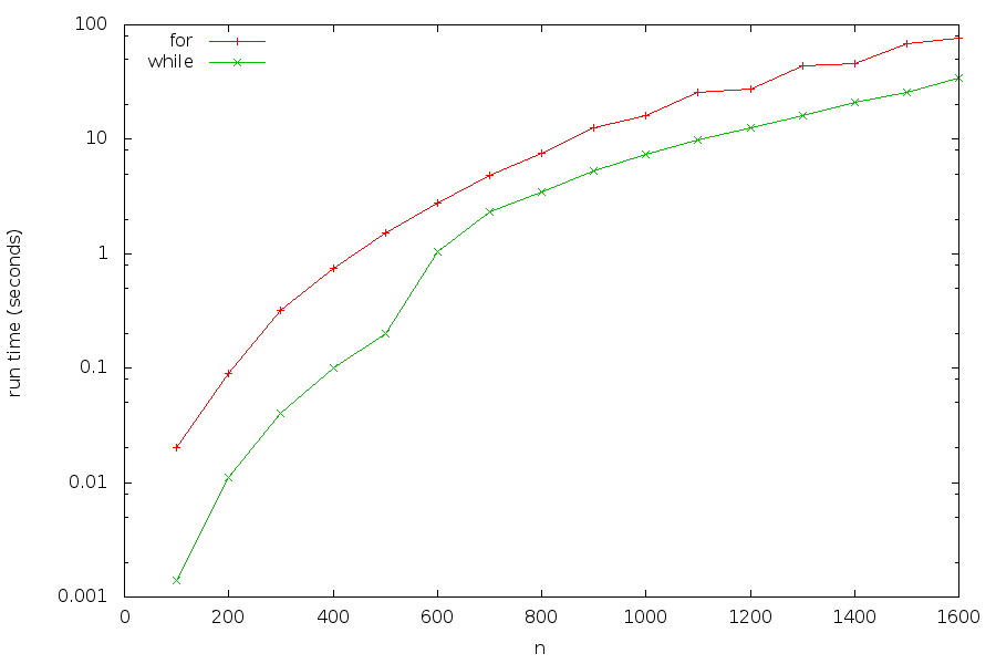
Performance-wise, we are happy with this first improvement (but do observe that the code is no longer as concise and readable as it was!).
Next, observe from the plot above that there is a non-uniform increase in run times around \(n=600\). One possible explanation is that the two matrices \(A\) and \(B\) alone start to fill the 6-megabyte L3 cache of the particular CPU microarchitecture on which the tests were run. In particular, the main memory bus bandwidth becomes a bottleneck which leads to a loss in performance. To alleviate this bottleneck, we use the knowledge that the bus is best utilized if we access memory at consecutive memory addresses. Indeed, the main memory serves the CPU with 512-bit cache lines (of 8 consecutive 64-bit words), and we obtain best bandwidth utilization by making use of all the 8 words that arrive via the memory bus to the CPU rather than one word (which happens if we access memory nonconsecutively with a stride of at least 8 words).
Let us now look at the code and put this knowledge into use.
First, observe that the inner loop accesses the matrix \(A\) (this)
by making accesses to consecutive words in the array this.entries.
Thus these accesses are not the bottleneck. However, the matrix
\(B\) (that) is accessed so that the elements
that(i,column) and that(i+1,column) are not consecutive
(at consecutive positions) in the underlying array that.entries.
We therefore do a slightly counter-intuitive trick:
we transpose (change the rows to columns and vice versa)
the matrix \(B\) before we execute the actual multiplication.
In this way, the elements of \(B\) considered in the inner loop are now
at consecutive memory addresses:
def transpose: Matrix =
  val r = new Matrix(n)
  for (row <- 0 until n; column <- 0 until n) do
    r(column, row) = this(row, column)
  r

def multiply_while_transpose(that: Matrix): Matrix =
  val that_tp = that.transpose
  val result = new Matrix(n)
  var row = 0
  while (row < n) do
    var column = 0
    while (column < n) do
      var v = 0.0
      var i = 0
      while (i < n) do
        v += this(row, i) * that_tp(column, i)
        i += 1
      end while
      result(row, column) = v
      column += 1
    end while
    row += 1
  end while
  result
end multiply_while_transpose
When we compare the performance, we get the following:
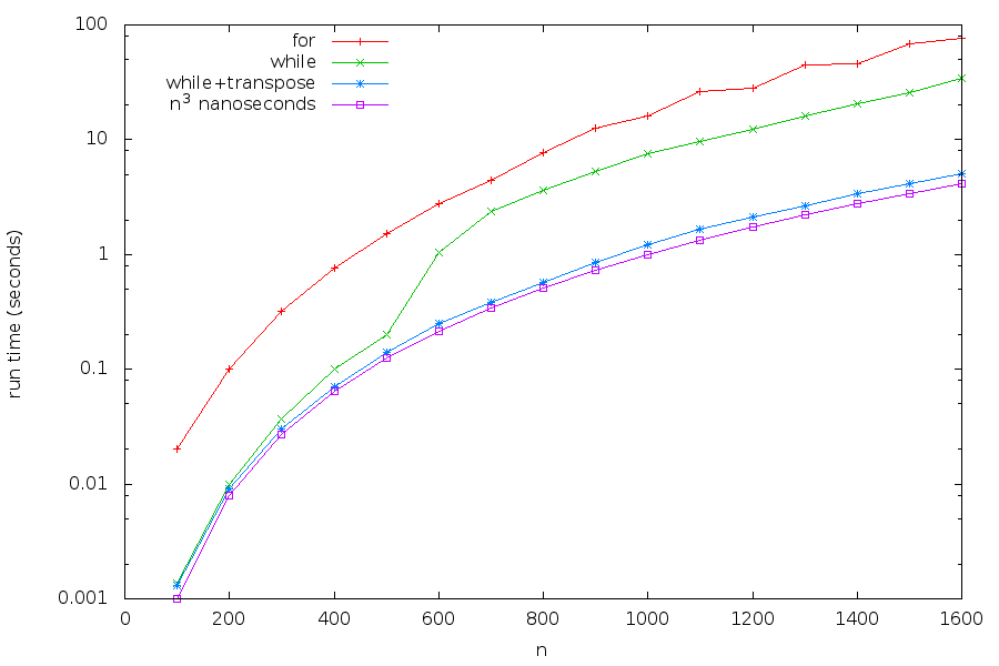
Thus we have obtained what is roughly a 10–30 times speedup compared with our original implementation of the same algorithm!
Observe that we have also plotted the function “\(n^3\) nanoseconds”
to give some perspective: the machine on which the tests were run
has clock rate of 3.1 GHz and therefore runs \(3.1\) clock cycles a nanosecond.
Recalling that multiplying \(n\)-by-\(n\) matrices with this algorithm must perform
\(n^3\) multiplications of type Double, the run time of our last
implementation is expected to be fairly close to an optimal one for
this algorithm in Scala. (Although further speedup could be obtained
by running the algorithm in parallel on multiple cores, and making use
of vectorization if supported by the CPU microarchitecture. Such
optimizations are likely to lead to yet more losses in readability,
maintainability, and portability.)
Optimize code only if absolutely necessary.
Note
Code optimization is sometimes useful, especially when something is done billions of times. But first find out whether the algorithms have the best possible scaling for the particular use case (for example, recall exponential vs almost linear in our earlier example of computing circuit values!). And as optimizations almost always degrade readability and thus maintainability of the code, only optimize the parts that are absolutely critical for performance. Use a profiling tool if available to find out the hotspots where most time is spent, and only then proceed to optimize these parts of your code. Fine-tuning the code for extreme performance typically requires detailed knowledge of the target CPU microarchitecture and the memory interface.