Case: Operations on matrices
Let us now proceed with a case study involving matrix computations.
Note
Recall that matrices are two-dimensional arrays of numbers that are routinely used in numerical computations ranging from data analysis to computer graphics. More precisely, an \(n\)-by-\(n\) matrix \(A\) is an array
whose entries \(a_{i,j}\) for \(1\leq i,j\leq n\) take values over, say, the real numbers. (Or for concrete numerical computations, IEEE 754-2019 floating point numbers.)
Let us recall the two basic arithmetic operations for matrices, namely the sum and the product of two matrices.
Note
For two \(n\)-by-\(n\) matrices, \(A\) and \(B\), the sum
is defined for all \(1\leq i,j\leq n\) by the rule
For example,
Note
For two \(n\)-by-\(n\) matrices, \(A\) and \(B\), the product
is defined for all \(1\leq i,j\leq n\) by the rule
For example,
We can implement matrices with these two basic operations as follows:
package matrices:

  /**
  * A simple class for square matrices with Double entries.
  */
  class Matrix(val n: Int):
    require(n > 0, "The dimension n must be positive")
    protected[Matrix] val entries = new Array[Double](n * n)

    /* With this we can access elements by writing M(i,j) */
    def apply(row: Int, column: Int) =
      require(0 <= row && row < n)
      require(0 <= column && column < n)
      entries(row * n + column)
    end apply

    /* With this we can set elements by writing M(i,j) = v */
    def update(row: Int, column: Int, value: Double) : Unit =
      require(0 <= row && row < n)
      require(0 <= column && column < n)
      entries(row * n + column) = value
    end update

    /* Returns a new matrix that is the sum of this and that */
    def +(that: Matrix): Matrix =
      val result = new Matrix(n)
      for row <- 0 until n; column <- 0 until n do
        result(row, column) = this(row, column) + that(row, column)
      result
    end +

    /* Returns a new matrix that is the product of this and that */
    def *(that: Matrix): Matrix =
      val result = new Matrix(n)
      for row <- 0 until n; column <- 0 until n do
        var v = 0.0
        for i <- 0 until n do
          v += this(row, i) * that(i, column)
        result(row, column) = v
      end for
      result
    end *

  end Matrix
Let us compare how well these methods scale when we increase the dimension \(n\) of the \(n\)-by-\(n\) matrix.
As a first try, we can execute some tests on random matrices manually. Open a console, import the contents of the matrices package, and then define the following function to build a random matrix:
import matrices._

val prng = new scala.util.Random(2105)
def randMatrix(n: Int) =
  val m = new Matrix(n)
  for(r <- 0 until n; c <- 0 until n) m(r, c) = prng.nextDouble()
  m
Now we can time how fast the addition and multiplication operators perform for a couple of different matrix sizes. First \(100 \times 100\):
scala> val a = randMatrix(100)
scala> val b = randMatrix(100)
scala> measureCpuTimeRepeated { val c = a + b }
res: (Unit, Double) = ((),1.6891891891891893E-4)
scala> measureCpuTimeRepeated { val c = a * b }
res: (Unit, Double) = ((),0.0125)
Then \(1000 \times 1000\):
scala> val a = randMatrix(1000)
scala> val b = randMatrix(1000)
scala> measureCpuTimeRepeated { val c = a + b }
res: (Unit, Double) = ((),0.015714285714285715)
scala> measureCpuTimeRepeated { val c = a * b }
res: (Unit, Double) = ((),16.59)
As programmers and aspiring practitioners of the scientific method we should of course seek to (i) automate our measurements, and (ii) run a systematic set of experiments.
A somewhat more systematic way to proceed is to implement a small tester object which generates pseudo-random \(n\)-by-\(n\) matrices for different values of \(n\) and applies the addition and multiplication methods on them.
You can find the code for this object matrices.compareAndPlot in the chapter source code package.
When we run the code, we witness the following printed in the Debug Console:
Measuring with n = 100
  Addition took 2.4154589371980676E-4 seconds
  Multiplication took 0.0125 seconds
.
.
.
Measuring with n = 900
  Addition took 0.01 seconds
  Multiplication took 12.78 seconds
Measuring with n = 1000
  Addition took 0.012222222222222223 seconds
  Multiplication took 16.15 seconds
Warning
The concrete measured run times of course may vary depending on the hardware, computer load, and so forth present if you choose to repeat this experiment yourself with your own hardware (classroom hardware) – which you should of course do!
To run the code yourself, open the project in VS Code (or your development environment of choice) and run compareAndPlot in src/…/compareAndPlot.scala.
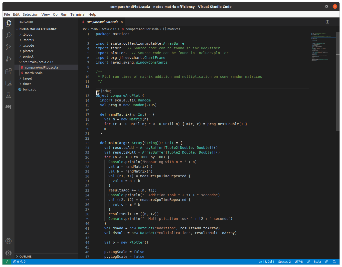
Run compareAndPlot to measure how long the matrix operators take to execute and plot the results.
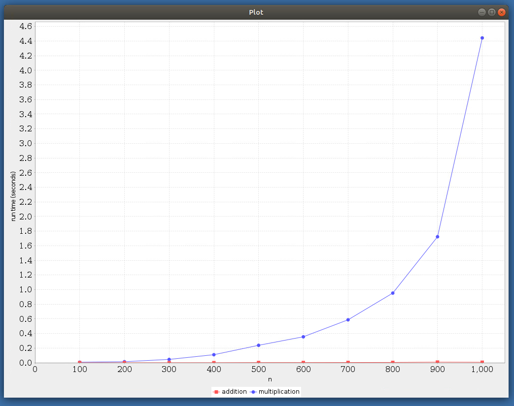
Matrix addition and multiplication efficiency (linear axis).
Observe that the time taken by matrix multiplication is much larger compared to that taken by addition. In particular, we cannot really distinguish the “addition” plot from the \(x\)-axis when the \(y\)-axis uses linear scale.
It might be better to compare the results by using a logarithmic scale on the \(y\)-axis.
You can tell the plotter to use a logarithmic scale for the \(y\)-axis by changing the line:
p.yLogScale = false
to:
p.yLogScale = true
in compareAndPlot.scala.
Re-run the program, and you will now see that the \(y\)-axis is using a log-scale, making it easier to compare the run-times.
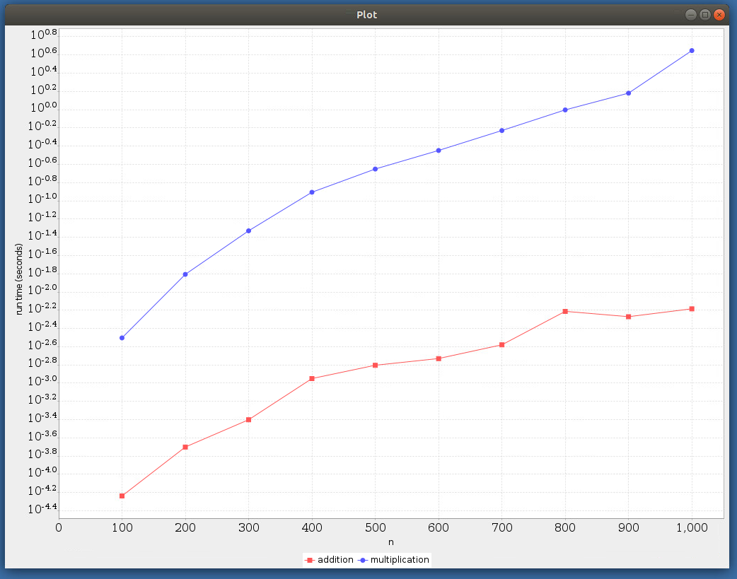
Matrix addition and multiplication efficiency (lin-log axis).
Observe the logarithmic scale on the y-axis. As expected, we witness that the matrix addition scales much better than multiplication.
When considering the scale of the run times it is useful to recognise that a 1600-by-1600 matrix has 2.56 million Double elements, thus taking about 20 megabytes of memory.
The small fluctuations in the run times are due to a large number of possible reasons, including
memory locality depending on currently active other processes,
random input enabling short-circuit evaluation to skip some of the recursions,
measurement inaccuracy,
and so forth.
Nevertheless, we observe that both addition and multiplication each present systematic scaling behaviour in their run times, and thus it pays off to try to understand precisely how and why such scaling arises, and in particular why the scaling is different for different functions.