Generalisation beyond presented examples
The gist of all learning from data is that the data contains useful regularity that can be automatically identified.
For example, from a human perspective the handwritten zeroes and ones are “clearly” different in our scanner output:
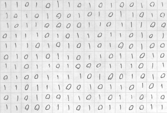
Thus we can argue that the scanner output in itself contains sufficient regularity for learning to succeed.
But how do we articulate this “difference” or “regularity” to a machine so that it can learn?
Let us adopt the role of a teacher instead of a programmer and think about the task.
Presented examples
To teach a topic, a key responsibility of a teacher is to select and prepare material to assist in learning. That is, a teacher prepares examples that the learner can then use to learn the topic at hand.
In our case, in terms of handwritten binary digits, it is of course our responsibility to present examples of what zero and one look like, in scanner output.
Towards this end, one possibility is simply to isolate parts of scanner output that contain individual digits, and label the isolated parts with the actual digit (either 0 or 1).
Below is a labeled dataset consisting of six digits in scanner output, each labeled with the actual digit (displayed in green) represented by the output.
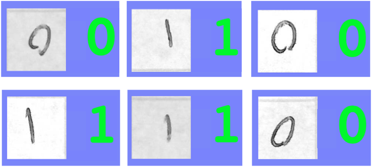
What we observe from the data is that no two examples are the same. Yet our hope and intuition is that by labeling enough data, it becomes possible to automatically tell apart between zeroes and ones. That is, the labeled data can be used to train the machine to tell the difference between a zero and a one.
Generalising into the unknown
The gist of learning is that we want to be able to generalise beyond the training data and obtain useful results on data that is unknown during training.

Comparing with the training set (the six labeled examples above), this example is not part of the training set, yet we would like the machine to automatically identify (or classify) the example as a zero. Indeed, intuitively the example above is “close enough” to the training data (especially if we had more training data available) so that it is not impossible to make the generalisation.
In concrete programming terms, in the exercises you are in fact encouraged to mimic this intuition of “closeness”, and classify previously unseen data based on the label of the nearest neighbour in the training data.
Remark. (*) In case you are interested, you can read more about classification in statistics and machine learning. (*)
The role of the programmer/teacher
In essence, we have now adopted an approach to programming where it is up to us to prepare a set of good examples (training data) that enables the machine to learn. The machine will then put in the effort to learn (to generalise) from the presented examples.
Our role has thus been reduced to that of a teacher. In essence, we need to prepare the training data so that the examples are
easy to learn, that is, the desired regularity is appropriately articulated, and
comprehensive, that is, the examples explore the desired regularity across the different contexts where we want successful generalisation to take place.
A common strategy is to assist/facilitate the learning by identifying features in the data that articulate the desired regularity and reduce the amount of data required for successful learning.
For example, in our handwritten digit example the data that we get and that the machine is supposed to classify is a 160-by-160 grayscale image that contains either a zero or a one. One approach to ease learning is to articulate the digit and to reduce the dimensionality in the data. We can accomplish this (a) by downsampling to 40-by-40, (b) by making the exposure uniform and thresholded (anything at most a fixed fraction of the average shade becomes black or otherwise white), and finally (c) by centering the thresholded image at the barycenter of the black pixels. This sequence of transformations (a,b,c) results in the following 40-by-40 feature vectors, highlighted with red:
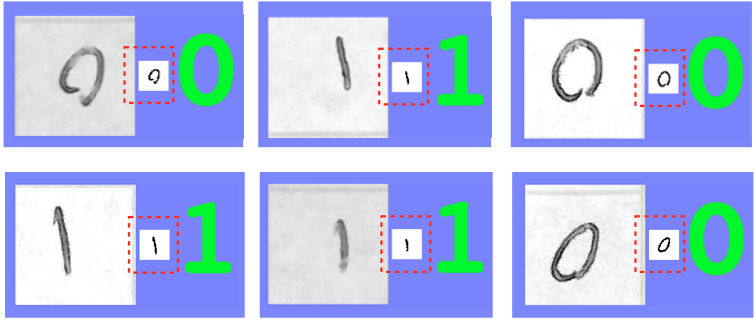
We observe that the feature vectors, arguably, and at least visually, “articulate” the zeroes and ones in the data, compared with the data available directly from the scanner.
Remark. (*) In case you are interested, you can read more about feature vectors in statistics and machine learning. (*)
Of course, an ideal situation is that we as programmers put very little effort into preparing the data for learning. Indeed, perhaps you can recognise that the task of classifying the handwritten digits into zeroes and ones is very, very easy. The bare minimum is just to base the classification on the amount of ink on the paper.
Remark 2. (**) Perhaps you want to challenge yourself to teach the machine to read handwritten decimal digits, as written by you? All you need is some square paper, fair handwriting skills, a scanner (or the camera in your handheld device), and a little bit of exploratory enthusiasm. Indeed, in programming terms this is not a great deal of work if you use the code already available to you. In handwriting terms, though, be prepared for hard labour. (**)
Testing
As soon as we have a framework of training the machine to generalise beyond presented examples, we should of course be interested in the quality of such generalisations.
For example, in terms of handwritten digits, we are naturally interested whether the machine can actually “see” the digits zero and one beyond the training data.
That is, we want to test our chosen framework of generalisation beyond the training data.
A simple strategy to test the ability to generalise is to split the available labeled data (the set of examples where we have available the correct class, or the label, of each example) randomly into two disjoint parts,
the training data (that we use for training the classifier), and
the test data (that we use to test whether the trained classifier outputs the correct label).
The fraction of correctly classified examples in the test data then gives a measure of the quality of the framework.
Remark. (*) The fraction of correctly classified examples is the accuracy of the classifier on the test data. Other useful concepts associated with binary classification are precision and recall. (*)
To validate the quality of a framework for classification, it makes sense to repeat the accuracy measurement for a number of random splits (into training/test data) and look at the distribution of accuracy values so obtained. A conservative strategy is to study the minimum accuracy across a large number of repetitions.
Remark. (*) What we have described above is essentially one-fold cross-validation. Follow the link for more about cross-validation in statistics (*).
Example. Suppose we have labels for the following handwritten digits.
We can now randomly split the handwritten digits into training data and test data.
Serendipity of a random split. Here it is useful to employ a random split to guarantee that a representative set of examples lands in both sets (training/test) in terms of scanner exposure, the position and size of the digit in the square, and other properties that vary across the data. In fact, assuming we have a large amount of data compared with the number of properties of interest, the random split guarantees that with high probability each property of interest is roughly equally represented in both sets (training/test).
Remark. (*) If you are familiar with probability, you may want to prove this claim for yourself in a more quantitative manner. (*)
Validation is important to guard against overfitting.
An inherent limitation of validation is that it is restricted to the available labeled data.
Let us next give a general discussion of risks and rewards of machine learning as a programming abstraction.